Note
Go to the end to download the full example code.
U.S. EIA: a week of real California generation#
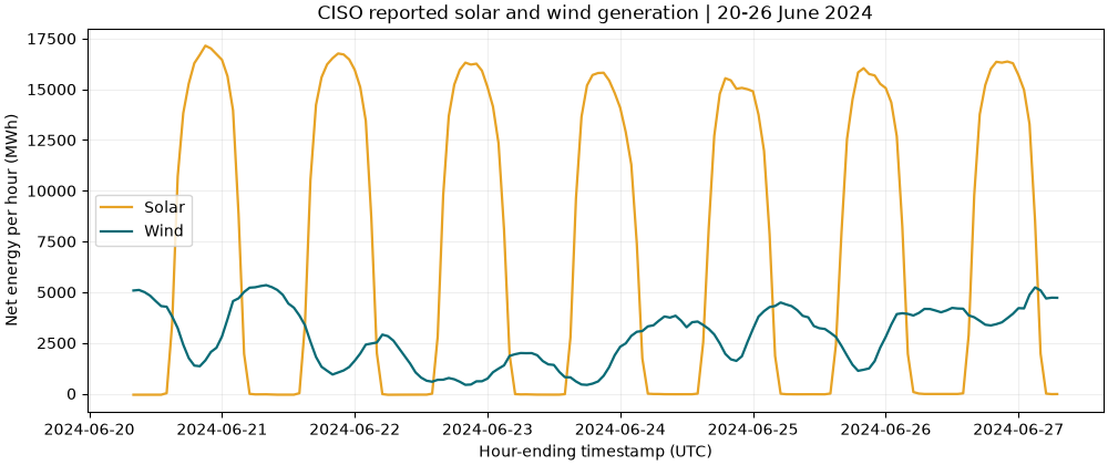
Parse 168 genuine hourly EIA-930 records for California ISO (CISO), 20-26 June 2024, and compare reported solar and wind output. The bundled CSV contains original rows from EIA’s public six-month balance file. No network or API key is used when building this gallery.
EIA-930 is system-level generation, not individual plant SCADA. Source coverage excludes much distributed generation. Data can be revised; the provenance file records the download date, exact source URL and checksums. See EIA’s coverage and time conventions.
Download the real CSV,
provenance manifest, or
all generation examples with their data.
1. Verify the captured official data#
The SHA-256 guards against accidentally changing the captured measurements. The original CSV header calls the hourly average power MW; the connector multiplies by the one-hour interval to report energy in MWh, matching the API’s energy units. It retains the original unit and value for inspection.
import hashlib
import json
from pathlib import Path

import matplotlib.pyplot as plt

from energy_data_retrieval.sources.eia import parse_balance_csv

example_directory = (
    Path(globals().get("__file__", Path.cwd() / "plot_generation_eia.py")).resolve().parent
)
data_directory = example_directory / "data"
sample = data_directory / "generation_eia_ciso_2024.csv"
manifest = json.loads(
    (data_directory / "generation_eia_ciso_2024.provenance.json").read_text(encoding="utf-8")
)
raw = sample.read_bytes()
assert hashlib.sha256(raw).hexdigest() == manifest["sample_sha256"]
print(f"Source: {manifest['source_url']}")
print(f"Captured: {manifest['retrieved_at_utc']}")
Source: https://www.eia.gov/electricity/gridmonitor/sixMonthFiles/EIA930_BALANCE_2024_Jan_Jun.csv
Captured: 2026-10-30T06:49:58.362106+00:00
2. Parse generation and inspect its physical meaning#
Source timestamps mark the end of each UTC hour. The explicit interval start avoids assigning the midnight hour to the wrong operating day. Missing observations remain missing, zero stays zero, and negative net generation is preserved. Imputed and adjusted columns are not substituted for reported data.
frame = parse_balance_csv(raw.decode("utf-8"), respondents=["CISO"], fuel_types=["SUN", "WND"])
print(frame[["timestamp", "area", "technology", "value", "unit", "source_unit"]].head())
print(f"Unique reported hour labels: {frame['timestamp'].nunique()}")
print(f"Missing selected fuel observations: {frame['value'].isna().sum()}")
                  timestamp  area technology   value unit source_unit
0 2024-06-20 08:00:00+00:00  CISO      Solar   -54.0  MWh          MW
1 2024-06-20 08:00:00+00:00  CISO       Wind  5083.0  MWh          MW
2 2024-06-20 09:00:00+00:00  CISO      Solar   -53.0  MWh          MW
3 2024-06-20 09:00:00+00:00  CISO       Wind  5109.0  MWh          MW
4 2024-06-20 10:00:00+00:00  CISO      Solar   -53.0  MWh          MW
Unique reported hour labels: 168
Missing selected fuel observations: 0
3. Plot the measured system profiles#
These are hourly net energy observations. They must not be interpreted as instantaneous power measurements or as the output of one solar/wind plant.
profiles = frame.pivot(index="timestamp", columns="fueltype", values="value")
colors = {"SUN": "#e7a326", "WND": "#096b76"}
names = {"SUN": "Solar", "WND": "Wind"}
fig, ax = plt.subplots(figsize=(10, 4.2), layout="constrained")
for code in ("SUN", "WND"):
    ax.plot(profiles.index, profiles[code], label=names[code], color=colors[code], linewidth=1.6)
ax.set(
    title="CISO reported solar and wind generation | 20-26 June 2024",
    xlabel="Hour-ending timestamp (UTC)",
    ylabel="Net energy per hour (MWh)",
)
ax.grid(alpha=0.2)
ax.legend()
plt.show()
4. Aggregate complete local operating days#
This specific summer week has 24 hours per California civil day. Requiring 24 nonmissing hourly values prevents a partial day from looking like a full day. A general workflow must calculate 23/24/25 expected hours at DST changes.
frame["operating_day"] = frame["interval_start_utc"].dt.tz_convert("America/Los_Angeles").dt.date
daily = frame.groupby(["operating_day", "fueltype"])["value"].sum(min_count=24).unstack()
fig, ax = plt.subplots(figsize=(9, 4.2), layout="constrained")
daily.rename(columns=names).plot.bar(
    ax=ax, color=[colors[code] for code in daily.columns], rot=25, width=0.8
)
ax.set(
    title="CISO complete local-day reported generation",
    xlabel="Operating day (America/Los_Angeles)",
    ylabel="Daily net energy (MWh)",
)
ax.grid(axis="y", alpha=0.2)
plt.show()
print(daily.round(1))
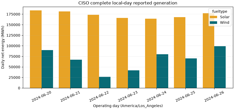
fueltype            SUN      WND
operating_day
2024-06-20     183654.0  89590.0
2024-06-21     181251.0  67108.0
2024-06-22     173346.0  26419.0
2024-06-23     165830.0  41750.0
2024-06-24     164303.0  79788.0
2024-06-25     168124.0  70334.0
2024-06-26     177256.0  99311.0
5. Retrieve your own observations#
The API supports bounded date and respondent filters and fetches all pages.
Register a free key at https://www.eia.gov/opendata/register.php and put it in
EIA_API_KEY. Do not paste keys into code, notebooks or committed output.
This block is an instruction, deliberately not executed during docs builds.
from datetime import UTC, datetime
from energy_data_retrieval.sources.eia import EIA_HOSTS, EIAClient
from energy_data_retrieval.transport import HTTPClient

with HTTPClient(EIA_HOSTS) as http:
    client = EIAClient.from_environment(http)
    result = client.hourly_generation(
        datetime(2024, 6, 20, 8, tzinfo=UTC),
        datetime(2024, 6, 27, 7, tzinfo=UTC),
        respondents=["CISO"],
        fuel_types=["SUN", "WND"],
    )
    print(result.frame.head())
For actual individual power plants, use EIA-923 monthly generation:
client.monthly_generation("2024-01", "2024-12", plant_codes=["YOUR_PLANT_CODE"]).
Use client.metadata("monthly") to inspect the official schema. Keep the
plant/fuel/prime-mover dimensions and select one aggregation level before
adding records, because aggregate ALL rows overlap their detail rows.
The key-free route is also a connector method:
EIAClient(http).balance_file(2024, 1, Path("balance.csv"), respondents=["CISO"]).
It downloads a full six-month file (tens of MB), retains the source and its
checksum manifest, and then filters the normalized observations locally.
Total running time of the script: (0 minutes 0.234 seconds)