Note
Go to the end to download the full example code.
Timestral for solar: an audited four-model win#
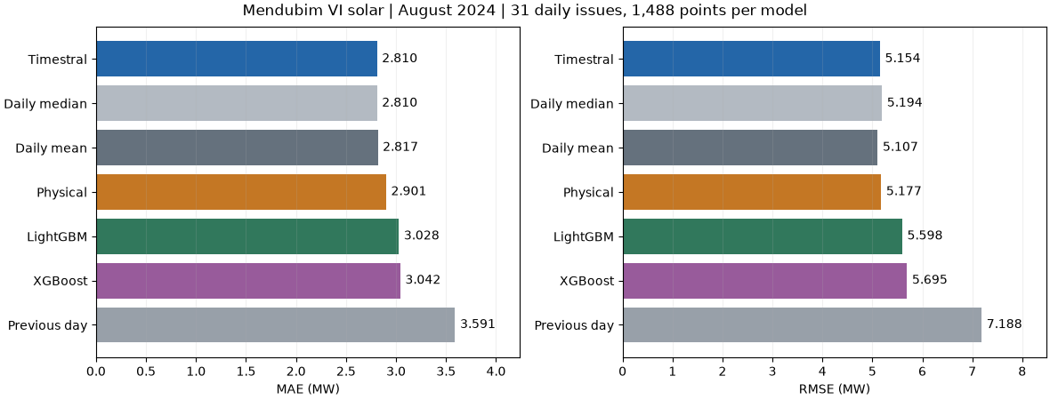
A real use case: 24-hour generation forecasts for Mendubim VI, Brazil, using ONS half-hour observations. Timestral-28M uses the preceding 14 days of generation, without weather forecasts or fine tuning. On all 31 August 2024 days, its MAE is lower than LightGBM, XGBoost and the physical surrogate by 7.2%, 7.6% and 3.1%, respectively.
The stronger-baseline check matters. Timestral is effectively tied with the 14-day same-clock median: 2.809545 versus 2.809680 MW MAE, a 0.0048% difference. The same-clock mean has better RMSE. This is a useful win over the three fitted comparators, not evidence that Timestral is meaningfully better than every model.
The plant was selected from 20 June candidates. After a failed July validation of Timestral-5M, June/July selected the final size and inputs; August was reserved for evaluation. The full search, failed attempt and subsequent data-availability repairs are disclosed in the case guide.
Research inspiration: Ascencio-Vásquez et al. (2020), Advanced PV Performance Modelling Based on Different Levels of Irradiance Data Accuracy, Energies 13(9), 2166, doi:10.3390/en13092166. Its attention to irradiance quality motivates the resource checks. This forecast comparison uses different data and models; it does not reproduce the paper’s experiment.
Download the runnable example and data,
scores and
selection audit.
Default execution is offline: fit the tree/physical models again and replay
checksum-verified actual Timestral inference, with no PyTorch requirement.
1. Reproduce every forecast and separate development from August#
Every method gets only pre-issue information. Physical/tree models use resource, clock and previous-day-power features as appropriate; Timestral uses generation history alone. Daily mean/median use all 14 preceding values at each clock time. All methods score the same future labels, including nights and restriction flags.
import json
import os
from pathlib import Path

import matplotlib.dates as mdates
import matplotlib.pyplot as plt

from energy_analysis.forecast_benchmark import TIMESTRAL_MANIFEST
from energy_analysis.timestral_solar_case import (
    CASE_MODELS,
    daily_errors,
    run_solar_case,
    solar_case_scores,
)
from energy_methods.timestral import TimestralConnector

directory = (
    Path(globals().get("__file__", Path.cwd() / "plot_timestral_solar_case.py")).resolve().parent
    / "data/timestral_solar"
)
manifest = json.loads((directory / TIMESTRAL_MANIFEST).read_text())
connector = None
if os.environ.get("ENERGY_TIMESTRAL_CASE_LIVE") == "1":
    connector = TimestralConnector(
        manifest["model_id"],
        revision=manifest["model_revision"],
        device=os.environ.get("ENERGY_TIMESTRAL_DEVICE", "cpu"),
        local_files_only=os.environ.get("ENERGY_TIMESTRAL_LOCAL_ONLY") == "1",
    )
print("Timestral:", "live inference" if connector else "verified real inference, offline replay")
print(f"Checkpoint: {manifest['model_id']} @ {manifest['model_revision']}")
predictions = run_solar_case(directory, connector=connector)
scores = solar_case_scores(predictions)
print(
    scores[["period", "model", "origins", "samples", "mae_mw", "rmse_mw"]]
    .round(6)
    .to_string(index=False)
)
holdout = predictions[predictions["period"] == "August holdout"]
table = scores[scores["period"] == "August holdout"].set_index("model").sort_values("mae_mw")
print("August MAE reduction against each comparator:")
for model in CASE_MODELS:
    if model != "Timestral":
        gain = 100 * (1 - table.loc["Timestral", "mae_mw"] / table.loc[model, "mae_mw"])
        print(f"  {model}: {gain:.4f}%")
print("The Daily median margin is a practical tie; Daily mean has lower RMSE.")
output = os.environ.get("ENERGY_TIMESTRAL_CASE_OUTPUT")
if output:
    Path(output).mkdir(parents=True, exist_ok=True)
    predictions.to_csv(Path(output) / "predictions.csv", index=False)
    scores.to_csv(Path(output) / "scores.csv", index=False)


def finish_figure(figure, name):
    if output:
        figure.savefig(Path(output) / f"{name}.png", dpi=160)
    plt.show()
Timestral: verified real inference, offline replay
Checkpoint: mistralai/Timestral-28M @ 49b26409ac87b5935539a5d8ffe7f397b720db47
        period        model  origins  samples   mae_mw  rmse_mw
August holdout   Daily mean       31     1488 2.817207 5.107030
August holdout Daily median       31     1488 2.809680 5.193739
August holdout     LightGBM       31     1488 3.028465 5.598410
August holdout     Physical       31     1488 2.900642 5.177469
August holdout Previous day       31     1488 3.590715 7.187679
August holdout    Timestral       31     1488 2.809545 5.154373
August holdout      XGBoost       31     1488 3.042184 5.694536
   Development   Daily mean       47     2256 3.187276 5.724243
   Development Daily median       47     2256 3.296498 6.048355
   Development     LightGBM       47     2256 3.645525 6.696321
   Development     Physical       47     2256 3.356899 5.962898
   Development Previous day       47     2256 3.706837 7.218382
   Development    Timestral       47     2256 3.136869 5.830417
   Development      XGBoost       47     2256 3.605862 6.572767
August MAE reduction against each comparator:
  Physical: 3.1406%
  LightGBM: 7.2287%
  XGBoost: 7.6471%
  Previous day: 21.7553%
  Daily mean: 0.2720%
  Daily median: 0.0048%
The Daily median margin is a practical tie; Daily mean has lower RMSE.
2. Include the stronger seasonal baselines in the headline result#
Lower errors are better. Identical labels at three decimals deliberately show how small the MAE advantage over Daily median is. Model defaults are unchanged from the existing benchmark; no competitor hyperparameters were tuned here.
colors = {
    "Timestral": "#2466a8",
    "Physical": "#c47724",
    "LightGBM": "#31785c",
    "XGBoost": "#985b9b",
    "Previous day": "#98a0a9",
    "Daily mean": "#65717d",
    "Daily median": "#b3bac2",
}
fig, axes = plt.subplots(1, 2, figsize=(11.8, 4.5), layout="constrained")
for ax, metric, label in zip(axes, ("mae_mw", "rmse_mw"), ("MAE (MW)", "RMSE (MW)"), strict=True):
    bars = ax.barh(table.index, table[metric], color=[colors[m] for m in table.index])
    ax.bar_label(bars, fmt="%.3f", padding=4)
    ax.invert_yaxis()
    ax.set(xlabel=label, xlim=(0, table[metric].max() * 1.18))
    ax.grid(axis="x", alpha=0.18)
fig.suptitle("Mendubim VI solar | August 2024 | 31 daily issues, 1,488 points per model")
finish_figure(fig, "model_comparison")
3. Show the whole holdout, including days Timestral loses#
A positive difference means Timestral had lower daily MAE. Daily results show variability hidden by a single monthly rank. This is descriptive evidence; there is no statistical-significance claim from this one plant and month.
daily = daily_errors(predictions)
daily = daily[daily["period"] == "August holdout"].pivot(
    index="issue_time", columns="model", values="error_mw"
)
fig, axes = plt.subplots(2, 1, figsize=(11.8, 6.2), sharex=True, layout="constrained")
for model in ("Timestral", "Physical", "Daily median"):
    axes[0].plot(daily.index, daily[model], label=model, color=colors[model], linewidth=1.6)
axes[0].set(ylabel="Daily MAE (MW)", title="All August forecasts")
axes[0].legend(ncols=3)
for model in ("Physical", "Daily median"):
    advantage = daily[model] - daily["Timestral"]
    axes[1].plot(daily.index, advantage, label=f"{model} minus Timestral", color=colors[model])
    print(f"Timestral lower daily MAE than {model}: {(advantage > 0).sum()}/31 days")
axes[1].axhline(0, color="#59636f", linewidth=0.8)
axes[1].set(ylabel="MAE difference (MW)", xlabel="Forecast issue label (UTC)")
axes[1].legend(ncols=2)
axes[1].xaxis.set_major_formatter(mdates.DateFormatter("%d %b"))
for ax in axes:
    ax.grid(alpha=0.18)
finish_figure(fig, "daily_comparison")
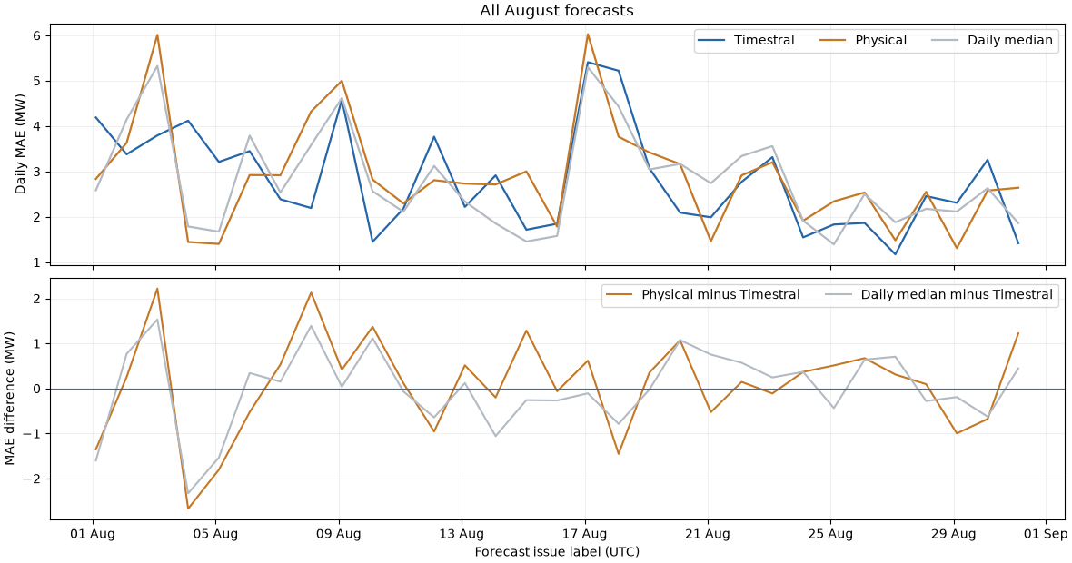
Timestral lower daily MAE than Physical: 19/31 days
Timestral lower daily MAE than Daily median: 16/31 days
4. Inspect the first three days, selected by date#
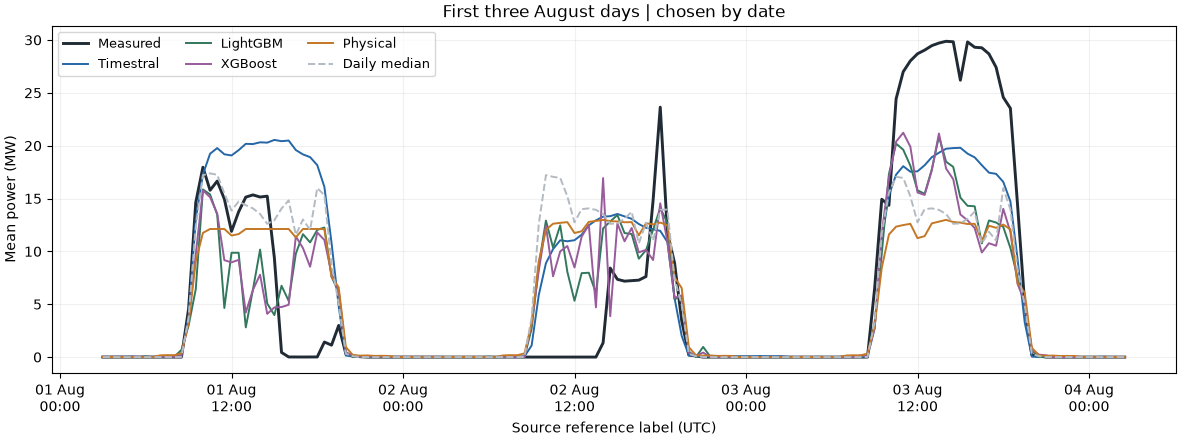
These forecasts are fixed for each 24-hour window. The plotted dates are not selected by favorable errors. Generation is mean MW, not half-hour MWh. Saved P10/P90 quantiles are model outputs, not calibrated confidence bounds.
first_issues = sorted(holdout["issue_time"].unique())[:3]
detail = holdout[holdout["issue_time"].isin(first_issues)]
actual = detail[detail["model"] == "Timestral"].sort_values("timestamp")
fig, ax = plt.subplots(figsize=(11.8, 4.4), layout="constrained")
ax.plot(actual["timestamp"], actual["actual_mw"], color="#202b35", label="Measured", linewidth=2.1)
for model in ("Timestral", "LightGBM", "XGBoost", "Physical", "Daily median"):
    rows = detail[detail["model"] == model].sort_values("timestamp")
    ax.plot(
        rows["timestamp"],
        rows["prediction_mw"],
        label=model,
        color=colors[model],
        linewidth=1.4,
        linestyle="--" if model == "Daily median" else "-",
    )
ax.set(
    title="First three August days | chosen by date",
    ylabel="Mean power (MW)",
    xlabel="Source reference label (UTC)",
)
ax.xaxis.set_major_formatter(mdates.DateFormatter("%d %b\n%H:%M"))
ax.legend(ncols=3, fontsize=9)
ax.grid(alpha=0.18)
finish_figure(fig, "first_three_days")
What this result supports#
A pretrained generation-only model is useful when reliable future weather is unavailable. Here it beats the three fixed fitted comparators, without local fitting or fine tuning, while simple seasonal forecasts remain competitive. The sensor gap explains the need for robust input handling, but this experiment does not isolate its causal contribution to the ranking. ONS data are revised historical records, future weather is persistence, the physical model is an isothermal surrogate, and Timestral pretraining overlap is unknown. Results do not establish universal superiority, operational savings or significance.
Total running time of the script: (0 minutes 4.352 seconds)