Note
Go to the end to download the full example code.
Brazil: measured generation and PV operating restrictions#
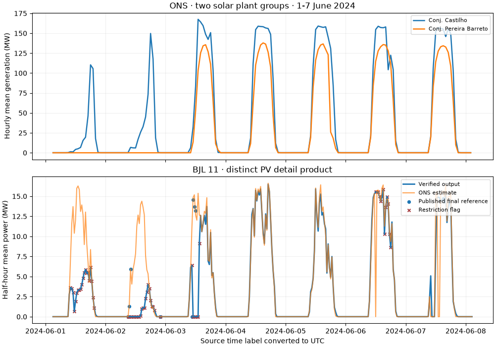
Read seven days of real ONS data: 336 hourly observations for two solar plant groups, plus 672 half-hour observations from the distinct photovoltaic constrained-off detail product. Actual output, estimated output and the final reference stay separate throughout the example.
Sources: ONS hourly generation
and ONS PV detail.
Download the hourly native CSV,
PV detail native CSV, and
capture manifest.
The gallery uses captured source measurements offline, without credentials.
import hashlib
import json
from pathlib import Path

import matplotlib.pyplot as plt

from energy_data_retrieval.sources.ons import parse_generation_csv
1. Verify the original CSV row selections#
Native semicolon CSV headers and complete rows are preserved byte for byte. Each manifest records the full downloaded source hash, selection and sample hash. A new bounded acquisition, outside this offline example, looks like:
from datetime import date
from energy_data_retrieval.sources.ons import ONS_HOSTS, ONSClient
from energy_data_retrieval.transport import HTTPClient
with HTTPClient(ONS_HOSTS) as http:
    client = ONSClient(http)
    result = client.generation(date(2024, 6, 1), date(2024, 6, 7),
                               plant_ids=["CJU_SPPB"])
    detail = client.solar_curtailment(date(2024, 6, 1), date(2024, 6, 7),
                                    plant_ids=["BAFB11"])
The client discovers Parquet exports through ONS’s catalogue; the gallery keeps small native CSV selections for transparent offline inspection.
directory = Path(globals().get("__file__", Path.cwd() / "plot_generation_ons.py")).resolve().parent
data = directory / "data"
frames = {}
for name, product in [
    ("generation_ons", "generation"),
    ("generation_ons_solar", "solar_curtailment"),
]:
    manifest = json.loads((data / f"{name}_provenance.json").read_text())
    raw = (data / manifest["fixture"]).read_bytes()
    if hashlib.sha256(raw).hexdigest() != manifest["fixture_sha256"]:
        raise ValueError("ONS capture differs from its provenance")
    frames[product] = parse_generation_csv(raw.decode("utf-8-sig"), product=product)
    print(product, "source:", manifest["source_url"])
    print("Captured:", manifest["retrieved_at_utc"], "rows:", len(frames[product]))
generation source: https://ons-aws-prod-opendata.s3.amazonaws.com/dataset/geracao_usina_2_ho/GERACAO_USINA-2_2024_06.csv
Captured: 2026-10-30T08:09:21.009740+00:00 rows: 336
solar_curtailment source: https://ons-aws-prod-opendata.s3.amazonaws.com/dataset/restricao_coff_fotovoltaica_detail_tm/RESTRICAO_COFF_FOTOVOLTAICA_DETAIL_2024_06.csv
Captured: 2026-10-30T08:09:21.502922+00:00 rows: 672
2. Keep source quantities and flags visible#
MWmed means average power in MW over the reporting interval. It is not MWh. The hourly product can contain plant groups; small-plant/MMGD estimates are excluded by default. Source clock labels are interpreted as Brazilian civil time here (UTC-03 in June 2024) and converted to UTC without shifting labels. The PV detail parser retains every source field, including invalid irradiance flags and null reference values.
hourly = frames["generation"]
solar = frames["solar_curtailment"]
plant = solar.loc[solar["unit_id"].eq("BAFB11")]
restricted = plant["flg_geracaorestrita"].astype(str).eq("1")
print("PV half-hours with a source restriction flag:", int(restricted.sum()))
print(
    "PV half-hours with a published final reference:", plant["val_geracaoreferenciafinal"].count()
)
PV half-hours with a source restriction flag: 63
PV half-hours with a published final reference: 8
3. Compare measured solar profiles and operational references#
A restriction flag records operating conditions. The gap between an estimated curve and measured power is not, by itself, measured curtailment energy. ONS’s final reference exists only for applicable restriction cases; NaN stays missing and is not drawn as zero.
fig, axes = plt.subplots(2, 1, figsize=(10, 7), sharex=True, layout="constrained")
for name, profile in hourly.groupby("nom_usina"):
    axes[0].plot(profile["timestamp"], profile["value"], label=name, linewidth=1.8)
axes[0].set_title("ONS · two solar plant groups · 1-7 June 2024")
axes[0].set_ylabel("Hourly mean generation (MW)")
axes[1].plot(plant["timestamp"], plant["value"], label="Verified output", linewidth=2)
axes[1].plot(plant["timestamp"], plant["val_geracaoestimada"], label="ONS estimate", alpha=0.7)
axes[1].scatter(
    plant["timestamp"], plant["val_geracaoreferenciafinal"], label="Published final reference", s=18
)
axes[1].scatter(
    plant.loc[restricted, "timestamp"],
    plant.loc[restricted, "value"],
    marker="x",
    s=18,
    color="#a63d40",
    label="Restriction flag",
)
axes[1].set(
    title="BJL 11 · distinct PV detail product",
    ylabel="Half-hour mean power (MW)",
    xlabel="Source time label converted to UTC",
)
for ax in axes:
    ax.grid(alpha=0.2)
    ax.legend(fontsize=8, loc="upper right")
plt.show()
Reuse#
Credit Operador Nacional do Sistema Elétrico (ONS), retain the capture dates
and source product, and identify any plant selection. Historical DST labels
require an explicit clock convention; ambiguous labels fail instead of being
guessed. PV capture manifest.
Total running time of the script: (0 minutes 0.224 seconds)