Note
Go to the end to download the full example code.
Japan offshore wind: when does CAPEX inflation break an investment case?#
News trigger: Reuters, 5 November 2026, reported Tokyo Gas withdrawing from an offshore wind project near Kashima Bay, citing rising costs: https://www.reuters.com/business/energy/tokyo-gas-withdraws-ibaraki-offshore-wind-project-2026-11-05/
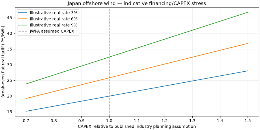
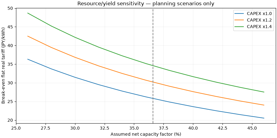
Business question: How do CAPEX inflation, net capacity factor, and real financing rates change the flat real electricity tariff needed to break even?
Evidence: A January 2026 Japan Wind Power Association (JWPA) planning scenario, presented at a Japanese METI committee meeting, provides generic fixed-bottom offshore-wind CAPEX, OPEX and capacity-factor assumptions. The numerical snapshot is attributed, NOT site-level observed project data. Other inputs are clearly labelled illustrative. No Kashima project’s actual costs, financing, bids, output or future viability are inferred.
Download the source assumptions and provenance. Method details and limitations:
offshore-wind economic stress guide.
from dataclasses import replace
from pathlib import Path

import matplotlib.pyplot as plt
import numpy as np

from energy_data_retrieval.cost_inputs import load_offshore_cost_snapshot
from energy_methods.offshore_wind_economics import (
    OffshoreWindScenario,
    evaluate_offshore_wind,
    tariff_npv_jpy,
)
1. Read an attributed 2026 industry planning scenario, offline#
The industry inputs are source-attributed figures, not measured generation. The scenario’s 25-year life, real rate of 6% and zero annual degradation are illustrative assumptions, not an interpretation of any project’s contract.
root = Path(globals().get("__file__", Path.cwd() / "plot_japan_offshore_wind_cost.py"))
source = root.resolve().parent / "jwpa_offshore_cost_2026.json"
benchmark = load_offshore_cost_snapshot(source)
scenario = OffshoreWindScenario(
    capacity_mw=100.0,
    capex_jpy_per_kw=benchmark.capex_jpy_per_kw,
    opex_jpy_per_kw_year=benchmark.opex_jpy_per_kw_year,
    net_capacity_factor=benchmark.net_capacity_factor,
    lifetime_years=25,
    discount_rate=0.06,
)
base = evaluate_offshore_wind(scenario)
print("Input evidence:", benchmark.evidence_class, benchmark.source_url)
print(f"Illustrative break-even real tariff: {base.lcoe_jpy_per_kwh:.1f} JPY/kWh")
print(f"Illustrative lifetime energy: {base.lifetime_energy_mwh / 1e3:.2f} GWh")
print("This is NOT an estimate of Kashima Bay LCOE or a JWPA model reproduction.")
Input evidence: published_industry_assumption https://www.meti.go.jp/shingikai/santeii/111.html
Illustrative break-even real tariff: 25.8 JPY/kWh
Illustrative lifetime energy: 8015.40 GWh
This is NOT an estimate of Kashima Bay LCOE or a JWPA model reproduction.
2. Plot sensitivity to capital-cost escalation and financing#
The dashed industry baseline represents assumed current CAPEX, not a reconstructed historical estimate or statistically observed probability.
multipliers = np.linspace(0.7, 1.5, 17)
real_rates = (0.03, 0.06, 0.09)
fig, ax = plt.subplots(figsize=(9, 4.5), layout="constrained")
for rate in real_rates:
    prices = [
        evaluate_offshore_wind(
            replace(
                scenario,
                capex_jpy_per_kw=scenario.capex_jpy_per_kw * factor,
                discount_rate=rate,
            )
        ).lcoe_jpy_per_kwh
        for factor in multipliers
    ]
    ax.plot(multipliers, prices, label=f"Illustrative real rate {rate:.0%}")
ax.axvline(1, linestyle="--", color="grey", label="JWPA assumed CAPEX")
ax.set(
    xlabel="CAPEX relative to published industry planning assumption",
    ylabel="Break-even flat real tariff (JPY/kWh)",
    title="Japan offshore wind — indicative financing/CAPEX stress",
)
ax.grid(alpha=0.2)
ax.legend()
plt.show()
3. Separate energy-resource sensitivity from investment cost#
Scenarios are not confidence intervals. Net capacity factor combines wind resource and technical losses; it is not an observed Kashima Bay series.
capacity_factors = np.linspace(0.26, 0.46, 11)
capex_increases = (1.0, 1.2, 1.4)
fig, ax = plt.subplots(figsize=(9, 4.5), layout="constrained")
for multiplier in capex_increases:
    prices = [
        evaluate_offshore_wind(
            replace(
                scenario,
                capex_jpy_per_kw=scenario.capex_jpy_per_kw * multiplier,
                net_capacity_factor=float(cf),
            )
        ).lcoe_jpy_per_kwh
        for cf in capacity_factors
    ]
    ax.plot(100 * capacity_factors, prices, label=f"CAPEX x{multiplier:.1f}")
ax.axvline(100 * benchmark.net_capacity_factor, linestyle="--", color="grey")
ax.set(
    xlabel="Assumed net capacity factor (%)",
    ylabel="Break-even flat real tariff (JPY/kWh)",
    title="Resource/yield sensitivity — planning scenarios only",
)
ax.grid(alpha=0.2)
ax.legend()
plt.show()
4. Audit cash-flow consistency with an assumed (NOT awarded) tariff#
The break-even tariff produces approximately zero NPV by construction. Compare it with a hypothetical 30 JPY/kWh flat real contract for an illustrative 100 MW asset; this is not a Japanese market price forecast.
hypothetical_tariff = 30.0
npv_jpy = tariff_npv_jpy(scenario, hypothetical_tariff)
print(f"At hypothetical {hypothetical_tariff:g} JPY/kWh: NPV = {npv_jpy / 1e9:.2f} bn JPY")
print(f"At break-even: NPV = {tariff_npv_jpy(scenario, base.lcoe_jpy_per_kwh):.2f} JPY")
At hypothetical 30 JPY/kWh: NPV = 17.23 bn JPY
At break-even: NPV = 0.00 JPY
Total running time of the script: (0 minutes 0.191 seconds)