Note
Go to the end to download the full example code.
Egypt wind financing: Niat and Rasgha bankability screening#
News (9 November 2026): Reuters reported a USD 436m financing package for the combined 500 MW Niat and Rasgha projects, with >2.3 TWh/year forecast, and an indicative USD 30/MWh power tariff.
Business decision: What generation, CAPEX and financing assumptions are implicit in the announcement? Which capacity-factor and interest-rate cases could cover an illustrative level debt payment?
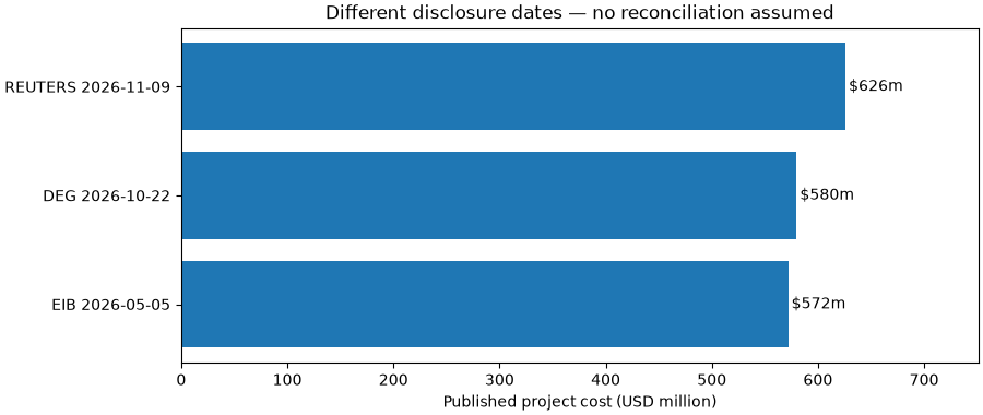
Evidence: Reuters (9 Nov), DEG (22 Oct), and EIB (5 May) report different
project-cost figures. These are separate, dated financing estimates, not
measured construction spending. Download the source-level evidence
snapshot. Details and limits: study guide.
NOT a valuation: No measured generation, published OPEX, actual loan repayment schedule, taxes, FX or debt covenants are available in these sources. Interest rates, loan tenor and OPEX below are ILLUSTRATIVE SCENARIOS, not terms agreed by the lenders. The >2.3 TWh claim is tested at 2.3 TWh as a conservative lower-bound proxy, not presented as an exact project forecast.
1. Reproduce reported source inputs with explicit dated provenance.#
import json
from dataclasses import replace
from pathlib import Path

import matplotlib.pyplot as plt
import numpy as np

from energy_methods.wind_project_finance import WindFinanceScenario, screen_wind_project

root = Path(globals().get("__file__", Path.cwd() / "plot_ras_ghareb_wind_finance.py"))
snapshot = root.resolve().parent / "ras_ghareb_wind_2026.json"
evidence = json.loads(snapshot.read_text(encoding="utf-8"))
claims = {item["source_id"]: item for item in evidence["reported_claims"]}
news = claims["reuters_20261109"]
assumptions = evidence["illustrative_assumptions"]
assert news["annual_generation_relation"] == "more_than"
assert news["finance_basis"] == "reported aggregate debt financing"

scenario = WindFinanceScenario(
    capacity_mw=news["rated_capacity_mw"],
    annual_generation_mwh=news["annual_generation_bound_mwh"],
    ppa_usd_per_mwh=news["ppa_usd_per_mwh_reported"],
    capex_usd=news["project_cost_usd"],
    senior_debt_usd=news["financing_usd"],
    annual_opex_usd=assumptions["opex_usd_per_kw_year"] * news["rated_capacity_mw"] * 1000,
    annual_interest_rate=assumptions["annual_interest_rate"],
    debt_tenor_years=assumptions["debt_tenor_years"],
)
base = screen_wind_project(scenario)
print("Reported forecast: MORE THAN 2.3 TWh/year, NOT measured generation.")
print(f"Implied net capacity factor: >{base.net_capacity_factor:.1%} (strict lower bound)")
print(f"At assumed flat 30 USD/MWh: >${base.gross_revenue_usd_year / 1e6:.1f}m/year gross")
print(f"Source-dated Reuters debt / CAPEX: {base.debt_to_capex:.1%}")
print("Illustrative interest 6%, 15-year amortization, OPEX $35/kW-year.")
print(f"Assumed annual debt payment: ${base.annual_debt_service_usd / 1e6:.1f}m")
print(f"Simplified cash cover at lower-bound energy: {base.cash_cover_ratio:.2f}x")
print("Not a lender-calculated DSCR; operating and contract terms are not verified.")
Reported forecast: MORE THAN 2.3 TWh/year, NOT measured generation.
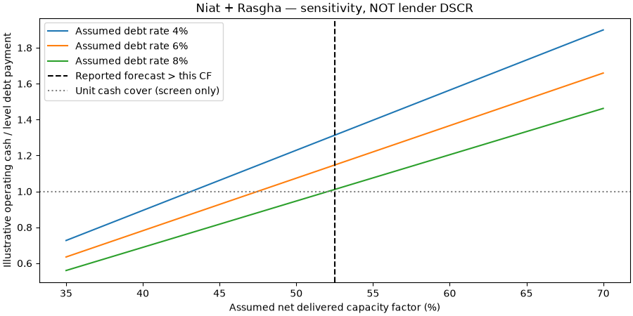
Implied net capacity factor: >52.5% (strict lower bound)
At assumed flat 30 USD/MWh: >$69.0m/year gross
Source-dated Reuters debt / CAPEX: 69.6%
Illustrative interest 6%, 15-year amortization, OPEX $35/kW-year.
Assumed annual debt payment: $44.9m
Simplified cash cover at lower-bound energy: 1.15x
Not a lender-calculated DSCR; operating and contract terms are not verified.
2. Finance sensitivity (no simulated measurements, no confidence intervals).#
capacity_factors = np.linspace(*assumptions["net_capacity_factor_sensitivity"], 41)
fig, ax = plt.subplots(figsize=(9, 4.5), layout="constrained")
for rate in assumptions["interest_rate_sensitivity"]:
    cover = [
        screen_wind_project(
            replace(
                scenario,
                annual_generation_mwh=scenario.capacity_mw * 8760 * float(cf),
                annual_interest_rate=rate,
            )
        ).cash_cover_ratio
        for cf in capacity_factors
    ]
    ax.plot(100 * capacity_factors, cover, label=f"Assumed debt rate {rate:.0%}")
ax.axvline(
    100 * base.net_capacity_factor,
    linestyle="--",
    color="black",
    label="Reported forecast > this CF",
)
ax.axhline(1, linestyle=":", color="gray", label="Unit cash cover (screen only)")
ax.set(
    xlabel="Assumed net delivered capacity factor (%)",
    ylabel="Illustrative operating cash / level debt payment",
    title="Niat + Rasgha — sensitivity, NOT lender DSCR",
)
ax.legend()
plt.show()
3. Preserve dated CAPEX disclosures instead of silently blending estimates.#
ordered = sorted(evidence["reported_claims"], key=lambda item: item["published_date"])
fig, ax = plt.subplots(figsize=(9, 3.8), layout="constrained")
labels = [f"{item['source_id'].split('_')[0].upper()} {item['published_date']}" for item in ordered]
capex = [item["project_cost_usd"] / 1e6 for item in ordered]
ax.barh(labels, capex)
for idx, value in enumerate(capex):
    ax.text(value + 3, idx, f"${value:.0f}m", va="center")
ax.set(
    xlim=(0, max(capex) * 1.2),
    xlabel="Published project cost (USD million)",
    title="Different disclosure dates — no reconciliation assumed",
)
plt.show()
Use this screen to identify due-diligence requests, not to approve lending: obtain P50/P90 net AEP, verified tariff/indexation, detailed debt schedule, curtailment, availability, insurance, OPEX, taxes and equity agreements. Reproduce offline: uv run –no-sync python examples/analysis/plot_ras_ghareb_wind_finance.py
Total running time of the script: (0 minutes 0.160 seconds)