Note
Go to the end to download the full example code.
From image candidates to a reproducible 3D PV scene near Rengo#
Continue the El Mirlo module-counting example: 2,055 candidate modules across 22 tables, in the same partial southern block. Their horizontal footprints are combined with a real Copernicus GLO-30 elevation crop and explicit mounting assumptions. This is 2.5D scenario geometry, not a photogrammetric reconstruction or an as-built survey.
The default assumes 20° tilt, local-north facing azimuth and 0.8 m minimum sampled terrain clearance. These values are not inferred from the image. One plane per table keeps adjacent modules aligned. The roughly 30 m DSM is interpolated for display; it cannot resolve module heights or foundations.
Download the offline viewer, OBJ/MTL meshes, full scene JSON,
source fixtures and runnable example.
The reusable method and other-site recipe explain coordinate conventions,
missing terrain, mounting choices and reproducibility.
Interactive scene#
Drag to orbit, scroll to zoom, and toggle terrain or modules in the legend. The initial view uses true metric proportions. The vertical-display control only changes presentation; exported coordinates always remain in metres.
Open the 3D viewer in a full window
The viewer embeds its chart library and requires a WebGL-capable browser. It uses no map tiles, external scripts or imagery texture. The static figures below and the OBJ/JSON exports remain available without WebGL.
import json
from pathlib import Path

import matplotlib.pyplot as plt
import numpy as np
from matplotlib.collections import PolyCollection
from matplotlib.patches import Rectangle

from energy_analysis.site_3d import footprints_from_count, plot_site_scene
from energy_analysis.site_3d.rengo import build_rengo_scene
from energy_analysis.site_3d.reports import scene_metadata
from energy_methods.pv_site_3d import MountingParameters, build_pv_site_scene

HERE = Path(globals().get("__file__", Path.cwd() / "example.py")).resolve().parent
study = build_rengo_scene(HERE / "data/rengo_modules", HERE / "data/rengo_3d")
scene = study["scene"]
source = study["terrain_source"]
window = study["terrain_window"]
credit = source["notice"]
summary = scene_metadata(scene)
print(
    json.dumps(
        {
            key: summary[key]
            for key in (
                "modelled_module_count",
                "modelled_table_count",
                "rejected_modules",
                "vertical_datum",
                "frame",
                "vertex_clearance_range_m",
            )
        },
        indent=2,
    )
)
{
  "modelled_module_count": 2055,
  "modelled_table_count": 22,
  "rejected_modules": [],
  "vertical_datum": "EGM2008",
  "frame": {
    "longitude": -70.8615,
    "latitude": -34.451499999999996,
    "elevation_origin_m": 282.0,
    "maximum_radius_m": 20000.0
  },
  "vertex_clearance_range_m": [
    0.8000000000000114,
    3.6698376975190854
  ]
}
1. Check the horizontal evidence and the native elevation grid#
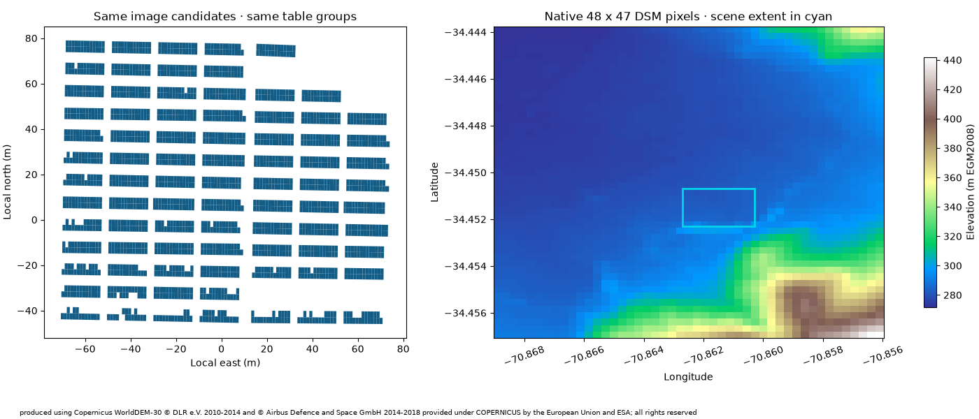
The original counter is re-run from its pinned image and configuration; accepted candidate IDs and table membership are retained. Its small audit matched 51 of 72 single-assistant reference centres on the development image, with no extras in those labelled regions. This is not independent field validation. No omitted modules or additional plant blocks are invented.
GLO-30 is a surface model, including vegetation and buildings. Its main acquisition predates the image; download time is not a survey date. Heights retain the EGM2008 vertical datum. The larger source crop shows context, while the cyan rectangle marks the much smaller model extent.
fig, axes = plt.subplots(1, 2, figsize=(14, 6), layout="constrained")
axes[0].add_collection(
    PolyCollection(
        [m.vertices_m[:, :2] for m in scene.modules], facecolors="#125c86", edgecolors="none"
    )
)
axes[0].autoscale()
axes[0].set_aspect("equal")
axes[0].set(
    title="Same image candidates · same table groups",
    xlabel="Local east (m)",
    ylabel="Local north (m)",
)
w, s, e, n = window.metadata.bounds
im = axes[1].imshow(
    window.elevation_m, extent=(w, e, s, n), interpolation="nearest", cmap="terrain", aspect="auto"
)
bw, bs, be, bn = scene.bounds_wgs84
axes[1].add_patch(Rectangle((bw, bs), be - bw, bn - bs, fill=False, ec="#00d5eb", lw=2))
axes[1].set(
    title="Native 48 x 47 DSM pixels · scene extent in cyan", xlabel="Longitude", ylabel="Latitude"
)
axes[1].ticklabel_format(useOffset=False, style="plain")
axes[1].tick_params(axis="x", rotation=20)
fig.colorbar(im, ax=axes[1], label="Elevation (m EGM2008)", shrink=0.8)
fig.text(0.02, 0.01, credit, fontsize=7, wrap=True)
fig.set_layout_engine("constrained", rect=(0, 0.08, 1, 0.9))
2. Build metric terrain and common table planes#
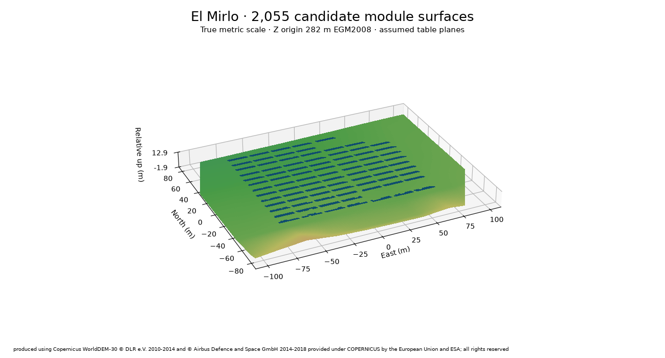
The generic method projects WGS84 footprints into a local azimuthal-equidistant frame. X is east, Y north and Z up; local Z=0 is 282 m EGM2008 here. A table’s tilt is absolute to horizontal. Its height is shifted until every sampled corner, edge midpoint and centre clears the source terrain by at least 0.8 m. This sampled condition is not a continuous-clearance or structural guarantee.
All 2,055 candidates have terrain support in this fixture. The display mesh has 81 x 121 interpolated vertices, which adds no native elevation detail.
fig = plot_site_scene(scene, title="El Mirlo · 2,055 candidate module surfaces", attribution=credit)
3. Show how an assumption changes the geometry#
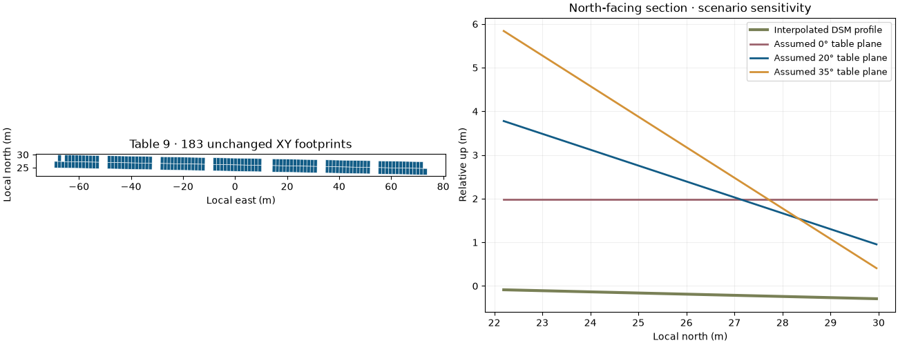
The same central table is rebuilt at 0°, 20° and 35°. Its horizontal footprint stays fixed; its slant dimensions therefore change with the assumed tilt. The common plane spans all candidates in the table, rather than restarting the tilt at each module. These curves illustrate model choices, not recovered measurements. The source profile passes through the table’s mean east coordinate.
footprints = footprints_from_count(study["counting"]["advanced"], scene.bounds_wgs84)
tables = sorted({f.table_id for f in footprints})
table_id = min(
    tables,
    key=lambda key: np.linalg.norm(
        np.concatenate([m.vertices_m[:, :2] for m in scene.modules if m.table_id == key]).mean(
            axis=0
        )
    ),
)
selected = [f for f in footprints if f.table_id == table_id]
fig, axes = plt.subplots(1, 2, figsize=(13, 5), layout="constrained")
base_xy = np.concatenate([scene.frame.project(f.vertices_wgs84) for f in selected])
axes[0].add_collection(
    PolyCollection(
        [scene.frame.project(f.vertices_wgs84) for f in selected],
        facecolors="#125c86",
        edgecolors="white",
        linewidths=0.4,
    )
)
axes[0].autoscale()
axes[0].set_aspect("equal")
axes[0].set(
    title=f"Table {table_id} · {len(selected)} unchanged XY footprints",
    xlabel="Local east (m)",
    ylabel="Local north (m)",
)
y = np.linspace(base_xy[:, 1].min(), base_xy[:, 1].max(), 100)
x = np.full_like(y, base_xy[:, 0].mean())
profile = study["grid"].sample(scene.frame.unproject(np.column_stack([x, y])))
axes[1].plot(
    y,
    profile - scene.frame.elevation_origin_m,
    color="#798056",
    lw=3,
    label="Interpolated DSM profile",
)
for tilt, colour in ((0, "#9c626c"), (20, "#125c86"), (35, "#d39237")):
    params = MountingParameters(tilt_degrees=tilt, azimuth_degrees=0, minimum_clearance_m=0.8)
    variant = build_pv_site_scene(
        selected,
        study["grid"],
        frame=scene.frame,
        bounds_wgs84=scene.bounds_wgs84,
        mounting=params,
        display_grid_shape=(11, 11),
    )
    corner = variant.modules[0].vertices_m[0]
    intercept = corner[2] - corner[:2] @ params.gradient
    heights = np.column_stack([x, y]) @ params.gradient + intercept
    axes[1].plot(y, heights, color=colour, lw=2, label=f"Assumed {tilt}° table plane")
axes[1].set(
    title="North-facing section · scenario sensitivity",
    xlabel="Local north (m)",
    ylabel="Relative up (m)",
)
axes[1].legend(fontsize=9)
axes[1].grid(alpha=0.2)
4. Export or reuse at another site#
export_site_scene writes viewer.html, site.obj / site.mtl,
scene.json and summary.json. The gallery download contains all of them.
JSON retains the CRS, height origin, vertical datum, source hashes, table IDs,
assumptions and rejected candidates. OBJ uses Z-up metres and contains surfaces,
not solid modules, support structures or surveyed foundations.
from energy_analysis.site_3d import export_site_scene
export_site_scene(
    scene, "outputs/el-mirlo-3d", title="El Mirlo inspection block",
    provenance={"terrain": source, "configuration": study["configuration"]},
    attribution=credit, evidence_note=study["configuration"]["assumptions_note"],
)
For another site, provide WGS84 quadrilateral module footprints with stable
feature IDs and a table property, a declared elevation raster and mounting
parameters. See the linked method guide for the complete runnable recipe.
No image-derived 3D depth, generation model or shading accuracy is claimed.
plt.show()
Total running time of the script: (0 minutes 1.506 seconds)