Note
Go to the end to download the full example code.
Brazil 2026 wind/PV curtailment: evidence audit and BESS screening limits#
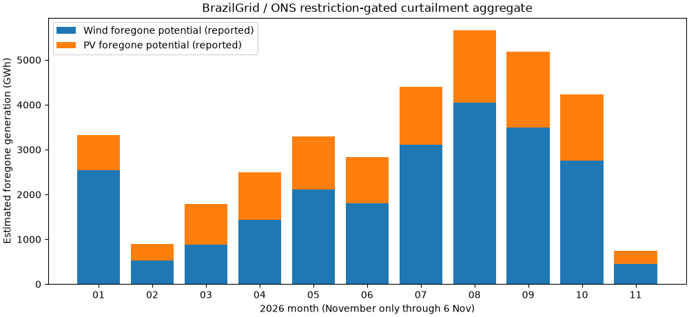
News trigger: The November 7, 2026 BrazilGrid Curtômetro update reports 34,850.8 GWh of foregone potential wind/PV output from January 1 through November 6, based on ONS reference generation and recorded restrictions. Wind: 23,132.0 GWh; solar: 11,718.8 GWh; an estimated 326.9 GWh is inside those totals. These are publisher-reported derived statistics, not directly metered production or independent reprocessing of ONS native records.
Business question: Which technology contributes most to exposure, and what does not follow from national curtailed-energy totals about BESS value?
Source (dated): https://brazilgrid.com/curtailment/brasil/
Underlying primary operator: https://dados.ons.org.br/
Method and scientific limits: docs/brazil-curtailment-screen.md.
import json
from pathlib import Path

import matplotlib.pyplot as plt

from energy_methods.curtailment_screen import (
    MonthlyCurtailment,
    audit_curtailment,
    hypothetical_deliverable_ceiling_gwh,
)
Frozen source PUBLISHED AGGREGATES; estimated subset included in wind+solar. Sphinx-Gallery may omit __file__: locate the project fixture offline.
script_path = Path(
    globals().get("__file__", Path.cwd() / "plot_brazil_curtailment_2026.py")
).resolve()
filename = "brazil_curtailment_ons_brazilgrid_20261107.json"
source = next(
    (
        path
        for ancestor in (script_path.parent, *script_path.parents)
        for path in (ancestor / filename, ancestor / "examples/analysis" / filename)
        if path.is_file()
    ),
    None,
)
if source is None:
    raise FileNotFoundError(f"Missing frozen attributed BrazilGrid summary {filename}")
data = json.loads(source.read_text(encoding="utf-8"))
rows = [
    MonthlyCurtailment(item["month"], item["wind"], item["solar"], item["estimated_subset"])
    for item in data["monthly_2026_gwh"]
]
current = data["reported_ytd_2026_gwh"]
prior = data["prior_matched_period_2025_gwh"]
audit = audit_curtailment(
    rows,
    reported_wind_gwh=current["wind"],
    reported_solar_gwh=current["solar"],
    reported_estimated_subset_gwh=current["estimated_subset"],
    prior_wind_gwh=prior["wind"],
    prior_solar_gwh=prior["solar"],
    display_precision_gwh=data["source"]["display_precision_gwh"],
)
print("PUBLISHED, not metered generation:", data["source"]["page_url"])
print(f"Cutoff date: {data['source']['observations_through']}; November is PARTIAL")
print(f"Curtailed potential wind + solar: {audit.reported_total_gwh / 1000:.3f} TWh")
print(f"Wind share: {audit.wind_share_pct:.1f}%; wind YoY: {audit.wind_yoy_pct:+.1f}%")
print(f"Solar YoY: {audit.solar_yoy_pct:+.1f}%; total YoY: {audit.total_yoy_pct:+.1f}%")
print(f"Estimated missing-data subset included in total: {audit.estimated_subset_pct:.2f}%")
print(f"Monthly rounding difference: {audit.reconciliation_difference_gwh:+.2f} GWh")
PUBLISHED, not metered generation: https://brazilgrid.com/curtailment/brasil/
Cutoff date: 2026-11-06; November is PARTIAL
Curtailed potential wind + solar: 34.851 TWh
Wind share: 66.4%; wind YoY: -1.9%
Solar YoY: +17.0%; total YoY: +3.7%
Estimated missing-data subset included in total: 0.94%
Monthly rounding difference: +0.10 GWh
These values are a secondary aggregation of ONS potential generation, NOT actually delivered wind/solar, nor investable storage energy.
fig, ax = plt.subplots(figsize=(10, 4.6), layout="constrained")
month_labels = [f"{row.month:02d}" for row in rows]
positions = list(range(len(rows)))
wind = [row.wind_gwh for row in rows]
solar = [row.solar_gwh for row in rows]
ax.bar(positions, wind, label="Wind foregone potential (reported)")
ax.bar(positions, solar, bottom=wind, label="PV foregone potential (reported)")
ax.set(
    xticks=positions,
    xticklabels=month_labels,
    xlabel="2026 month (November only through 6 Nov)",
    ylabel="Estimated foregone generation (GWh)",
    title="BrazilGrid / ONS restriction-gated curtailment aggregate",
)
ax.legend()
plt.show()
Purely HYPOTHETICAL physical upper bounds, with NO site, time or price data. This is not a dispatch model and not a prediction of achievable recovery.
fractions = [0.0, 0.01, 0.02, 0.05, 0.10]
round_trip_efficiency = 0.90  # HYPOTHETICAL battery parameter, not observed
ceilings = [
    hypothetical_deliverable_ceiling_gwh(
        audit.reported_wind_gwh,
        accessible_fraction=fraction,
        round_trip_efficiency=round_trip_efficiency,
    )
    for fraction in fractions
]
fig, ax = plt.subplots(figsize=(8.7, 4.3), layout="constrained")
ax.plot([100 * x for x in fractions], [x / 1000 for x in ceilings], marker="o")
ax.set(
    xlabel="Assumed fraction of foregone wind potential chargeable (%) — hypothetical",
    ylabel="Upper-bound battery delivery (TWh, 90% hypothetical RTE)",
    title="Illustrative ceiling only — NOT feasible dispatch or BESS revenue",
)
plt.show()
print(
    "Hypothetical 5% capture / 90% RTE ceiling:",
    f"{ceilings[3] / 1000:.3f} TWh; NO spatial/temporal feasibility evidence",
)
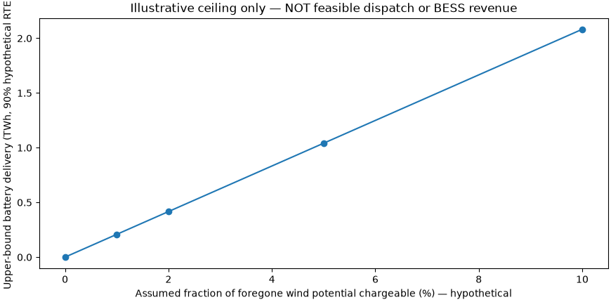
Hypothetical 5% capture / 90% RTE ceiling: 1.041 TWh; NO spatial/temporal feasibility evidence
Reproduce offline: uv run –no-sync python examples/analysis/plot_brazil_curtailment_2026.py To evaluate an actual BESS business case requires ONS half-hourly restriction intervals, site-level available generation, co-location/export constraints, cycle/calendar aging, charging availability and settled electricity prices.
Total running time of the script: (0 minutes 0.161 seconds)