Note
Go to the end to download the full example code.
Canary Islands: PVDeg thermal screening at 100 m#
For moisture, damp heat, light-assisted stress and solder fatigue, open the nine-map degradation-mechanism atlas.
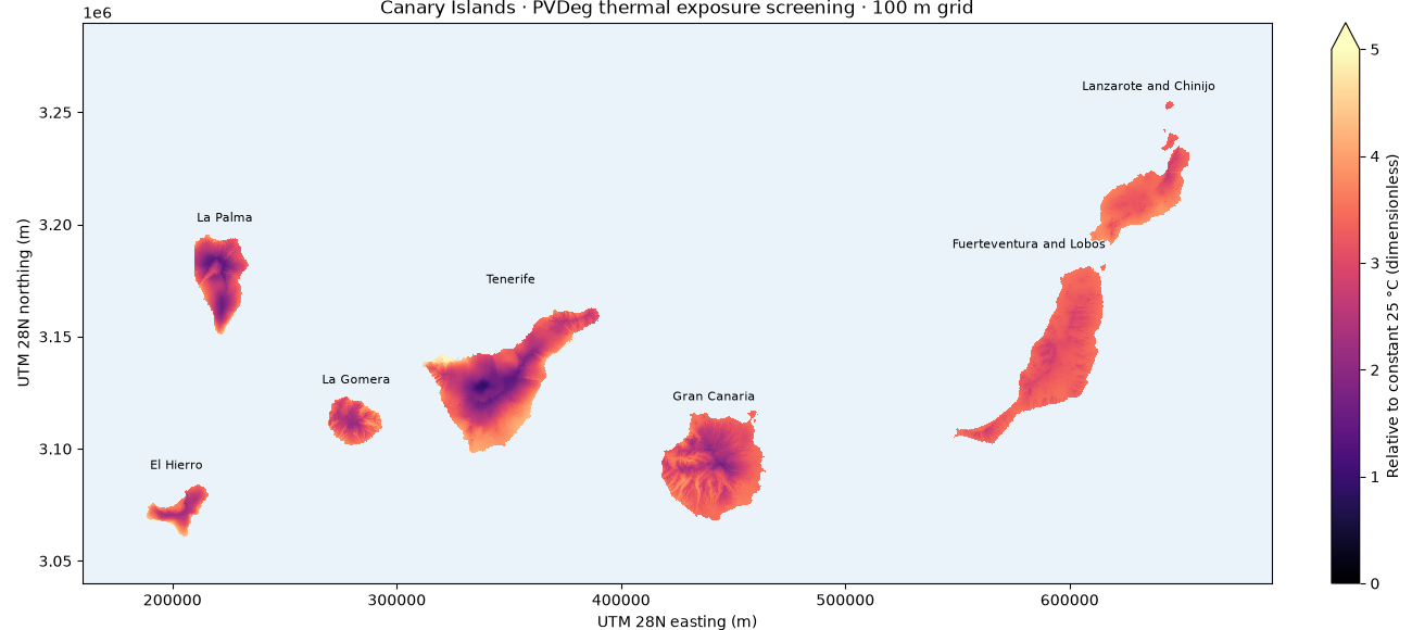
Real CHELSACanaryClim monthly temperature normals (1979-2013) drive the imported
pvdeg Python library. A 100 m projected grid covers all eight main islands,
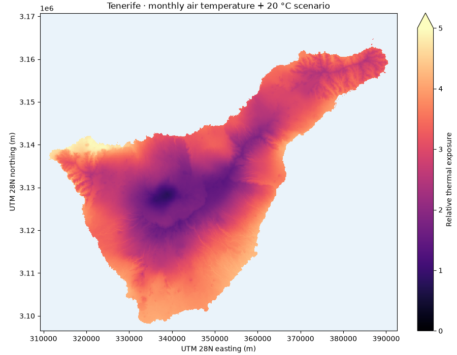
including La Graciosa. The color is relative Arrhenius thermal exposure, not
annual degradation, remaining life or measured module performance.
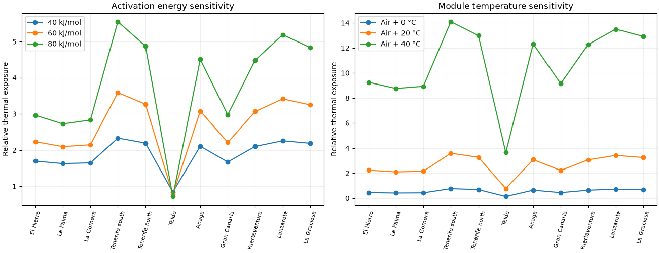
A constant +20 C module-air offset and 60 kJ/mol activation energy are screening assumptions. Humidity and irradiance effects are disabled. Monthly means miss hourly temperature peaks. See the guide for equations, limitations, source attribution and full reproduction commands.
Download provenance and inputs:
El Hierro,
La Palma,
La Gomera,
Tenerife,
Gran Canaria,
Fuerteventura,
Lanzarote and La Graciosa.
Place these beside the script to run offline. No synthetic climate is used.
import hashlib
import json
from pathlib import Path

import matplotlib.pyplot as plt
import numpy as np
import pandas as pd
from matplotlib.colors import Normalize
from rasterio.plot import plotting_extent

from energy_analysis.pvdeg_canary import MONTH_HOURS, screen_climate_tile
from energy_methods.pvdeg import thermal_stress_index
Recalculate the map with the actual PVDeg library#
manifest = json.loads(Path("pvdeg_canary_provenance.json").read_text())
results = {}
for island, record in manifest["tiles"].items():
    path = Path(record["file"])
    if hashlib.sha256(path.read_bytes()).hexdigest() != record["sha256"]:
        raise ValueError("Climate tile differs from its provenance")
    results[island] = screen_climate_tile(path)
print("Evidence: modeled 1979-2013 climatology → scenario thermal exposure")
print("Grid: 100 m EPSG:32628; no claim of 100 m PV degradation accuracy")
print("Valid land cells:", sum(np.isfinite(values).sum() for values, _ in results.values()))
Evidence: modeled 1979-2013 climatology → scenario thermal exposure
Grid: 100 m EPSG:32628; no claim of 100 m PV degradation accuracy
Valid land cells: 742013
All islands, with consistent colors#
fig, ax = plt.subplots(figsize=(13, 5.8), layout="constrained")
ax.set_facecolor("#eaf3fa")
norm = Normalize(0, 5)
for island, (values, profile) in results.items():
    extent = plotting_extent(values, profile["transform"])
    artist = ax.imshow(
        np.ma.masked_invalid(values),
        extent=extent,
        origin="upper",
        cmap="magma",
        norm=norm,
        interpolation="nearest",
    )
    ax.text(
        (extent[0] + extent[1]) / 2,
        extent[3] + 3000,
        manifest["tiles"][island]["label"],
        ha="center",
        fontsize=8,
    )
ax.set_xlim(160000, 690000)
ax.set_ylim(3040000, 3290000)
ax.set(
    xlabel="UTM 28N easting (m)",
    ylabel="UTM 28N northing (m)",
    title="Canary Islands · PVDeg thermal exposure screening · 100 m grid",
)
fig.colorbar(artist, ax=ax, label="Relative to constant 25 °C (dimensionless)", extend="max")
Tenerife: inspect the spatial detail#
values, profile = results["tenerife"]
fig, ax = plt.subplots(figsize=(9, 7), layout="constrained")
ax.set_facecolor("#eaf3fa")
artist = ax.imshow(
    np.ma.masked_invalid(values),
    extent=plotting_extent(values, profile["transform"]),
    cmap="magma",
    norm=norm,
    interpolation="nearest",
)
ax.set(
    title="Tenerife · monthly air temperature + 20 °C scenario",
    xlabel="UTM 28N easting (m)",
    ylabel="UTM 28N northing (m)",
)
fig.colorbar(artist, ax=ax, label="Relative thermal exposure", extend="max")
Sensitivity: scenario choices matter#
Existing attributed source samples are independent spot checks of climate diversity, not calibration or field validation of degradation.
samples = pd.read_csv("kgpv_canary_samples.csv")
air = samples[[f"t{m:02d}" for m in range(1, 13)]].to_numpy().T
fig, axes = plt.subplots(1, 2, figsize=(13, 5), layout="constrained")
for energy in (40, 60, 80):
    index = thermal_stress_index(air + 20, MONTH_HOURS, activation_energy_kj_mol=energy)
    axes[0].plot(samples["name"], index, "o-", label=f"{energy} kJ/mol")
for offset in (0, 20, 40):
    index = thermal_stress_index(air + offset, MONTH_HOURS)
    axes[1].plot(samples["name"], index, "o-", label=f"Air + {offset} °C")
for ax, title in zip(
    axes, ("Activation energy sensitivity", "Module temperature sensitivity"), strict=True
):
    ax.set(title=title, ylabel="Relative thermal exposure")
    ax.tick_params(axis="x", rotation=75, labelsize=8)
    ax.legend()
    ax.grid(alpha=0.2)
plt.show()
Total running time of the script: (0 minutes 4.244 seconds)