Note
Go to the end to download the full example code.
Bruna: frontal progression and Tenerife energy impact maps#
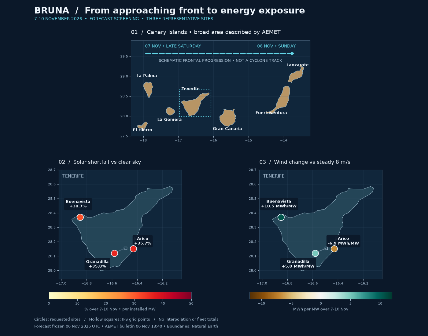
A geographic companion to Bruna: Tenerife solar and wind forecast impact. The top map shows the schematic west-to-east progression of the frontal weather, based on AEMET’s 6 November 2026 13:40 bulletin: western islands late Saturday 7 November, spreading across the archipelago on Sunday 8 November. The arrow is a directional illustration, not a cyclone-centre track. Highlighted islands show the broad bulletin scope, not an official warning polygon or uniform impact severity. A verified storm track would require time-stamped pressure-centre coordinates; none are inferred here from the three weather samples.
The lower maps show forecast energy at three representative Tenerife locations for 7-10 November, from the frozen pre-event IFS snapshot. Solar colour is the percentage shortfall against clear sky, not measured or causally attributed storm loss. Wind colour is signed MWh/MW against an assumed steady 8 m/s. Hollow squares show actual model grid coordinates linked to requested sites; there is no spatial interpolation or invented island-wide impact surface.
Boundaries: Natural Earth 1:10 million, public domain. Weather: Open-Meteo /
ECMWF, CC BY 4.0. Map geometry and provenance are in data/bruna; see
bruna_map_provenance.json for the bulletin, boundary URL, extraction rule and
checksums. This example runs offline. Run with
uv run python examples/analysis/plot_bruna_impact_maps.py.
import hashlib
import json
from pathlib import Path

import matplotlib.pyplot as plt
import numpy as np
import pandas as pd
from matplotlib.colors import Normalize, TwoSlopeNorm
from matplotlib.patches import Polygon, Rectangle

from energy_methods.storm_energy import storm_energy

example_dir = Path(__file__).resolve().parent if "__file__" in globals() else Path.cwd()
root = example_dir / "data" / "bruna"
meta = json.loads((root / "bruna_map_provenance.json").read_text())
geometry = (root / "bruna_islands.geojson").read_bytes()
assert hashlib.sha256(geometry).hexdigest() == meta["subset_sha256"]
islands = json.loads(geometry)["features"]
weather = pd.read_csv(root / "bruna_forecast.csv", parse_dates=["timestamp"])
records = json.loads((root / "bruna_provenance.json").read_text())["records"]
rows = []
for record in records:
    result = storm_energy(weather.loc[weather.site == record["site"]])
    reference = result.pv_reference_mwh_per_mw.sum()
    rows.append(
        {
            **record,
            "solar_shortfall": -100 * result.pv_delta_mwh_per_mw.sum() / reference,
            "wind_delta": result.wind_delta_mwh_per_mw.sum(),
        }
    )

navy, ocean, ink, muted = "#0b1829", "#10263b", "#eef5fc", "#aac0d4"
fig = plt.figure(figsize=(14, 11), facecolor=navy)
grid = fig.add_gridspec(2, 2, height_ratios=[0.85, 1.15], hspace=0.30, wspace=0.17)
regional = fig.add_subplot(grid[0, :])
solar = fig.add_subplot(grid[1, 0])
wind = fig.add_subplot(grid[1, 1])


def basemap(ax, bounds, fill):
    """Draw preserved geographic rings in a local lon/lat view."""
    ax.set_facecolor(ocean)
    for feature in islands:
        ring = np.asarray(feature["geometry"]["coordinates"][0])
        ax.add_patch(Polygon(ring, facecolor=fill, edgecolor="#9ab8c9", linewidth=0.8))
    ax.set(xlim=bounds[:2], ylim=bounds[2:])
    ax.set_aspect(1 / np.cos(np.deg2rad(28.4)))
    ax.tick_params(colors=muted, labelsize=8)
    ax.grid(color="#456078", alpha=0.22, linewidth=0.6)
    for spine in ax.spines.values():
        spine.set_color("#385168")


basemap(regional, (-18.35, -13.25, 27.5, 29.9), "#b79565")
labels = [
    ("El Hierro", -18.02, 27.62),
    ("La Palma", -17.90, 28.98),
    ("La Gomera", -17.25, 27.88),
    ("Tenerife", -16.65, 28.65),
    ("Gran Canaria", -15.60, 27.65),
    ("Fuerteventura", -14.35, 28.05),
    ("Lanzarote", -13.60, 29.25),
]
for name, lon, lat in labels:
    regional.text(lon, lat, name, color=ink, fontsize=9, ha="center", weight="bold")
regional.annotate(
    "",
    xy=(-13.65, 29.57),
    xytext=(-17.95, 29.57),
    arrowprops=dict(arrowstyle="-|>", color="#62d4e6", lw=3, linestyle="--"),
)
regional.text(-17.95, 29.72, "07 NOV • LATE SATURDAY", color="#62d4e6", fontsize=10)
regional.text(-13.65, 29.72, "08 NOV • SUNDAY", color="#62d4e6", fontsize=10, ha="right")
regional.text(
    -15.8,
    29.36,
    "SCHEMATIC FRONTAL PROGRESSION • NOT A CYCLONE TRACK",
    color=muted,
    fontsize=9,
    ha="center",
)
regional.add_patch(
    Rectangle(
        (-16.97, 27.98), 0.9, 0.68, fill=False, edgecolor="#62d4e6", linewidth=1.5, linestyle=":"
    )
)
regional.set_title(
    "01  /  Canary Islands • broad area described by AEMET",
    color=ink,
    loc="left",
    fontsize=13,
    pad=15,
)

for ax, column, cmap, norm, title, unit in [
    (
        solar,
        "solar_shortfall",
        "YlOrRd",
        Normalize(0, 50),
        "02  /  Solar shortfall vs clear sky",
        "% over 7-10 Nov • per installed MW",
    ),
    (
        wind,
        "wind_delta",
        "BrBG",
        TwoSlopeNorm(vmin=-12, vcenter=0, vmax=12),
        "03  /  Wind change vs steady 8 m/s",
        "MWh per MW over 7-10 Nov",
    ),
]:
    basemap(ax, (-17.02, -16.05, 27.94, 28.70), "#244557")
    for row in rows:
        x, y = row["requested_longitude"], row["requested_latitude"]
        gx, gy = row["grid_longitude"], row["grid_latitude"]
        ax.plot([x, gx], [y, gy], color=muted, lw=1, linestyle=":")
        ax.scatter(gx, gy, s=45, marker="s", facecolors="none", edgecolors=muted, zorder=3)
        points = ax.scatter(
            x,
            y,
            c=[row[column]],
            cmap=cmap,
            norm=norm,
            s=230,
            edgecolor=ink,
            linewidth=1.3,
            zorder=4,
        )
        offset = {"Buenavista": (-5, 23), "Arico": (22, 10), "Granadilla": (-40, -34)}
        suffix = "%" if column == "solar_shortfall" else " MWh/MW"
        ax.annotate(
            f"{row['site']}\n{row[column]:+.1f}{suffix}",
            (x, y),
            xytext=offset[row["site"]],
            textcoords="offset points",
            color=ink,
            fontsize=9,
            weight="bold",
            ha="center",
            bbox=dict(boxstyle="round,pad=0.4", fc=navy, ec="none", alpha=0.9),
        )
    ax.set_title(title, color=ink, loc="left", fontsize=12, pad=14)
    bar = fig.colorbar(points, ax=ax, orientation="horizontal", fraction=0.055, pad=0.10)
    bar.set_label(unit, color=muted, fontsize=9)
    bar.ax.tick_params(colors=muted, labelsize=8)
    bar.outline.set_edgecolor("#385168")
    ax.text(0.03, 0.96, "TENERIFE", transform=ax.transAxes, color=muted, fontsize=11, va="top")

fig.suptitle(
    "BRUNA  /  From approaching front to energy exposure",
    color=ink,
    fontsize=21,
    weight="bold",
    x=0.08,
    ha="left",
    y=0.98,
)
fig.text(
    0.08,
    0.94,
    "7-10 NOVEMBER 2026  •  FORECAST SCREENING  •  THREE REPRESENTATIVE SITES",
    color="#62d4e6",
    fontsize=10,
)
fig.text(
    0.08,
    0.025,
    "Circles: requested sites   /   Hollow squares: IFS grid points   /   "
    "No interpolation or fleet totals\n"
    "Forecast frozen 06 Nov 2026 UTC • AEMET bulletin 06 Nov 13:40 • Boundaries: Natural Earth",
    color=muted,
    fontsize=9,
    linespacing=1.7,
)
fig.subplots_adjust(top=0.88, bottom=0.11, left=0.08, right=0.95)
plt.show()
Total running time of the script: (0 minutes 0.245 seconds)