Note
Go to the end to download the full example code.
NIST: import measured photovoltaic testbed exports#
The NIST PV portal provides measured data from ground-mounted, rooftop and canopy arrays in Gaithersburg, Maryland. This example documents and executes the native export import workflow. Its default figure is a field guide, with no invented or downloaded generation observations.
Download a one-minute CSV through the portal, then run:
NIST_PV_CSV=/path/to/export.csv NIST_PV_ARRAY=ground uv run python examples/connectors/plot_generation_nist.py
The connector accepts ordinary CSV and Campbell TOA5 headers, preserves original
columns and records the file’s SHA-256. Portal accounts or transient download
tokens are not stored in the project. The script is included in the
generation example bundle.
1. Select the published AC power channel and time convention#
The NIST data paper specifies Eastern
Standard Time throughout the year, with no daylight-saving shift.
InvPAC_kW_Avg is one-minute average inverter AC power in kW; the unsuffixed
InvPAC_kW is a one-second instantaneous channel. Accumulated InvEtot_kWh
readings are a different physical quantity and are never treated as power.
import os
from pathlib import Path

import matplotlib.pyplot as plt

from energy_data_retrieval.sources.nist import NISTClient

export_path = os.environ.get("NIST_PV_CSV")
array = os.environ.get("NIST_PV_ARRAY", "ground")
2. Import real observations when a local provider export is supplied#
NAN readings remain missing. Negative/anomalous measurements remain as
reported. The parser verifies kW and Avg metadata in TOA5 files and refuses
conflicting duplicate timestamps. No interval-edge convention is invented.
if export_path:
    result = NISTClient().read_export(Path(export_path), array=array)
    frame = result.frame
    fig, ax = plt.subplots(figsize=(10, 4), layout="constrained")
    ax.plot(frame.timestamp, frame.value, color="#176e76", linewidth=0.9)
    ax.set(
        title=f"NIST {array}: imported measured one-minute AC power",
        ylabel="AC power [kW]",
        xlabel="UTC (source clock is fixed EST)",
    )
    print("Imported observations:", len(frame), "Input SHA-256:", frame.attrs["input_sha256"])
else:
    fig, ax = plt.subplots(figsize=(10, 4.5), layout="constrained")
    ax.axis("off")
    rows = [
        ["Download", "Choose Ground, Roof or Canopy in the NIST PV portal"],
        ["Power", "One-minute: InvPAC_kW_Avg [kW]"],
        ["Clock", "Fixed Eastern Standard Time = UTC-05:00"],
        ["Import", "NISTClient().read_export(path, array='ground')"],
        ["Provenance", "Original fields, input filename and SHA-256 retained"],
    ]
    table = ax.table(cellText=rows, colWidths=[0.18, 0.82], cellLoc="left", loc="center")
    table.auto_set_font_size(False)
    table.set_fontsize(10)
    table.scale(1, 2.1)
    ax.set_title("NIST PV: offline export guide — no measurements bundled", pad=20)
    print("Set NIST_PV_CSV to a real provider export to produce a measured power plot.")
plt.show()
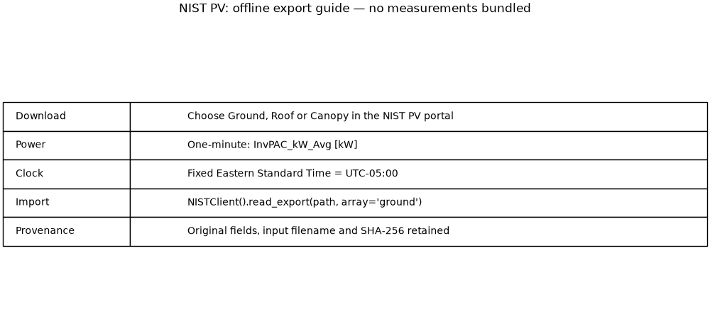
Set NIST_PV_CSV to a real provider export to produce a measured power plot.
3. Distinguish higher-frequency data and multiple channels#
For one-second exports, explicitly select power_column='InvPAC_kW' and
resolution='one-second'. Meter power PwrMtrP_kW_Avg is also supported.
A selected inverter/meter channel is not automatically the sum of every
inverter in an array. Check the downloaded table and NIST instrument metadata.
Total running time of the script: (0 minutes 0.064 seconds)