Note
Go to the end to download the full example code.
PVGIS 6: coverage, terrain and PV time series#
Work through real version 6 responses for the same Tenerife coordinate, with source availability, terrain context and an hourly PV calculation. All figures use preserved public API captures; the documentation makes no live requests.
The connector guide maps all 27 version 6
operations, including multiple surfaces, optimisation, solar position, TMY,
reference metadata and seven multipart POST variants. Download the
runnable examples and captures.
from pathlib import Path

import matplotlib.pyplot as plt
import pandas as pd

from energy_data_retrieval.sources.pvgis import describe_endpoint, endpoints, load_response
1. Discover the API contract and query source coverage first#
No key is needed. Run this code explicitly when acquiring fresh data:
from energy_data_retrieval.transport import HTTPClient
from energy_data_retrieval.sources.pvgis import PVGIS6Client, PVGIS_HOSTS
with HTTPClient(PVGIS_HOSTS) as http:
    api = PVGIS6Client(http)
    sources = api.available_sources(28.4775, -16.3294)
    terrain = api.elevation(28.4775, -16.3294)
    horizon = api.horizon(28.4775, -16.3294, angle_output_units="Degrees")
    power = api.power(28.4775, -16.3294, verbose=1,
                      start_time="2020-06-01T00:00:00",
                      end_time="2020-06-02T00:00:00")
    conventions = api.conventions()
    power.save(Path("my_power.json"))
Unlike PVGIS 5 aspect, version 6 surface orientation is north=0°. Requested
geometry is in degrees, while many returned angles default to radians. Use
verbose=1 for power timestamps and intermediate quantities.
print("Supported v6 operations:", *endpoints("6"), sep="\n")
print(
    "Irradiance-source options:",
    describe_endpoint("/power/broadband")["parameters"]["irradiance_source"],
)
folder = Path(globals().get("__file__", Path.cwd() / "plot_pvgis_v6.py")).resolve().parent
responses = {
    name: load_response(folder / "data" / f"pvgis_v6_{name}.json")
    for name in ("sources", "elevation", "horizon", "power", "degree_days")
}
print("Available sources:", responses["sources"].json())
print("Terrain metadata:", responses["elevation"].json())
print("Request parameters:", responses["power"].request.parameters)
Supported v6 operations:
GET /coverage/map
GET /coverage/layers
GET /coverage/layers/{name}
GET /coverage/location-within-selected-source
GET /coverage/available-sources-in-selected-location
GET /performance/broadband
POST /performance/broadband
GET /performance/broadband-multiple-surfaces
POST /performance/broadband-multiple-surfaces
GET /power/broadband
POST /power/broadband
GET /power/broadband-multiple-surfaces
POST /power/broadband-multiple-surfaces
GET /power/surface/optimisation
POST /power/surface/optimisation
GET /reference/citation
GET /reference/publications
GET /reference/conventions-in-pvgis
GET /reference/license
GET /solar-position/overview
POST /solar-position/overview
GET /features
GET /topography/horizon-profile
POST /topography/horizon-profile
GET /topography/elevation
GET /meteorological/typical-meteorological-year
GET /meteorological/degree-days
Irradiance-source options: {'type': 'string', 'enum': ['SARAH-3', 'ERA5', 'CLEAR-SKY [Hofierka et al. (2002)]'], 'default': 'SARAH-3'}
Available sources: {'irradiance_sources': ['SARAH-3', 'ERA5', 'CLEAR-SKY [Hofierka et al. (2002)]']}
Terrain metadata: {'latitude': 0.4970261377366852, 'longitude': -0.28500179487516203, 'elevation': 613.0}
Request parameters: {'method': 'GET', 'query:latitude': '28.4775', 'query:longitude': '-16.3294', 'query:start_time': '2020-06-01T00:00:00', 'query:end_time': '2020-06-02T00:00:00', 'query:verbose': '1'}
2. Inspect the source terrain horizon in requested angular units#
The horizon response’s reference string describes its origin/convention. Keep the elevation as a DEM value, not a surveyed module height.
horizon = responses["horizon"].json()["horizon_profile"]
print("Horizon reference:", horizon["reference"])
fig, ax = plt.subplots(figsize=(9, 4), layout="constrained")
ax.fill_between(horizon["azimuth"], horizon["horizon_height"], color="#64748b", alpha=0.6)
ax.set(
    title="PVGIS 6 · Tenerife terrain horizon",
    xlabel="Azimuth (degrees, north origin)",
    ylabel="Horizon height (degrees)",
)
ax.grid(alpha=0.2)
plt.show()
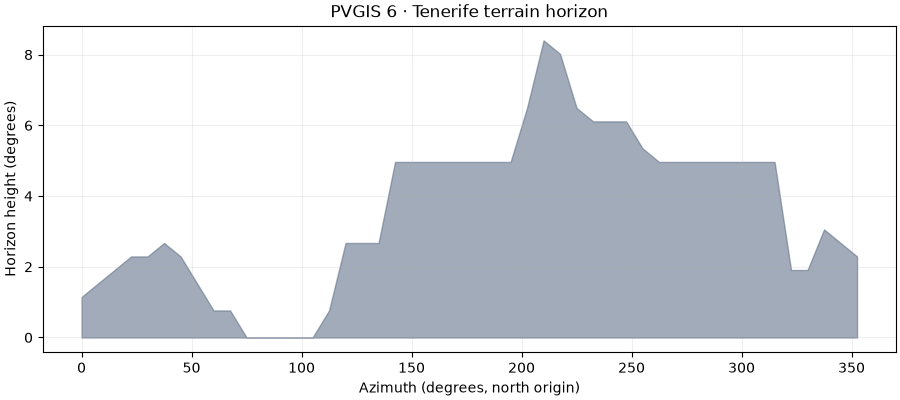
Horizon reference: Azimuth starts at North and increases clockwise
3. Preserve all native fields, selecting only the columns needed for plotting#
The complete payload contains geometry, model identifiers and intermediate
calculations alongside arrays. columns= selects a rectangular table
without discarding the original metadata. Times below are interpreted as UTC
because this exact saved request uses the provider’s UTC default. The provider
offsets timestamps within the hour; these values are displayed unchanged.
native = responses["power"].json()
frame = responses["power"].table(columns=("timestamps", "power", "global_inclined_irradiance"))
time = pd.to_datetime(frame["timestamps"], utc=True)
print("Peak capacity:", native["peak_power"], native["peak_power_unit"])
print("Technology and model:", native["technology"], native["power_model"])
print("Native geometry:", native["surface_tilt"], native["surface_orientation"], native["unit"])
fig, axes = plt.subplots(2, 1, figsize=(10, 6.5), sharex=True, layout="constrained")
axes[0].plot(time, frame["power"], color="#15803d", linewidth=2)
axes[0].set(title="PVGIS 6 · modelled hourly PV output, June 1-2, 2020", ylabel="PV power (W)")
axes[1].plot(time, frame["global_inclined_irradiance"], color="#d97706", linewidth=2)
axes[1].set(xlabel="Returned source timestamp (UTC)", ylabel="In-plane irradiance (W/m²)")
for ax in axes:
    ax.grid(alpha=0.2)
plt.show()
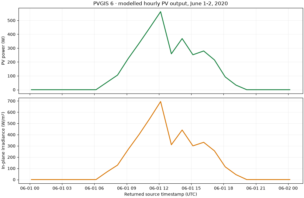
Peak capacity: 1 kWp
Technology and model: cSi:Free standing 2025 Huld 2011
Native geometry: 0.7853981633974483 3.141592653589793 radians
4. Add weather context, custom horizons and multi-surface designs#
The degree-day capture spans only June 1-3. Its monthly-labelled result is a partial-period calculation, so it cannot be treated as a complete June total.
print("Partial-period degree-day response:", responses["degree_days"].json())
#
# Other supported calls (run explicitly with your own data)::
#
#     # Uploaded file: JSON {"horizon_height": [0, 5, 10, 0], "units": "degrees"}
#     result = api.horizon(28.4775, -16.3294,
#                          horizon_file=Path("horizon.json"), angle_output_units="Degrees")
#     # Equal-length lists; peak power is kWp per surface.
#     result = api.multiple_surface_power(28.4775, -16.3294,
#         surface_tilt=[25, 25], surface_orientation=[90, 270],
#         start_time="2020-06-01T00:00:00", end_time="2020-06-02T00:00:00",
#         **{"peak-power": [1, 1]})
#     # Native text exports preserve provider headers and metadata.
#     result = api.typical_year(28.4775, -16.3294, epw="weather.epw")
#     result.save(Path("weather.epw"))
#
# Supplying a horizon file chooses POST automatically and places every input in
# the multipart body. No query/body assumptions are borrowed from version 5.
# Compare scenarios only after aligning time windows, sources, geometry, module
# technology, loss assumptions and units. A different version is not a field
# validation of another version's model.
Partial-period degree-day response: {'heating_days': {'2020-06': 0.0}, 'cooling_days': {'2020-06': 0.0}, 'average_temperature': {'2020-06': 18.814}, 'average_heating_days': 0.0, 'average_cooling_days': 0.0, 'mean_temperature': 18.814, 'temperature_output_units': 'Celsius'}
Total running time of the script: (0 minutes 0.211 seconds)