Note
Go to the end to download the full example code.
Failure rates, Bayesian updates and censored survivors#
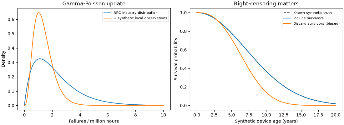
The left panel compares the NRC pump population distribution with an update from synthetic independent local observations. This is a method demonstration, not a measured improvement. The right panel uses a deterministic synthetic Weibull population to show why censored survivors must be retained.
import matplotlib.pyplot as plt
import numpy as np
from scipy.stats import gamma

from energy_data_retrieval.failure_database import load_failure_database
from energy_methods.failure_rates import GammaRate, fit_weibull_censored

source = load_failure_database("nrc_2020").set_index("failure_mode").loc["MDP-FTR-NR"]
prior = GammaRate(source.parameter1, source.parameter2)
posterior = prior.update(failures=2, exposure=2_000_000)  # synthetic local device-hours
fig, axes = plt.subplots(1, 2, figsize=(11, 4), layout="constrained")
rate = np.linspace(0, 10, 300)  # per million hours
for label, model in [
    ("NRC industry distribution", prior),
    ("+ synthetic local observations", posterior),
]:
    density = gamma.pdf(rate / 1e6, model.shape, scale=1 / model.rate) / 1e6
    axes[0].plot(rate, density, label=label)
axes[0].set(xlabel="Failures / million hours", ylabel="Density", title="Gamma-Poisson update")
axes[0].legend(fontsize=8)

q = (np.arange(1000) + 0.5) / 1000
lifetimes = 10 * np.sqrt(-np.log1p(-q))
failed = lifetimes <= 12
fit = fit_weibull_censored(np.minimum(lifetimes, 12), failed)
biased = fit_weibull_censored(lifetimes[failed], np.ones(failed.sum()))
age = np.linspace(0, 20, 100)
axes[1].plot(age, np.exp(-((age / 10) ** 2)), "k--", label="Known synthetic truth")
axes[1].plot(age, np.exp(fit.log_survival(age)), label="Include survivors")
axes[1].plot(age, np.exp(biased.log_survival(age)), label="Discard survivors (biased)")
axes[1].set(
    xlabel="Synthetic device age (years)",
    ylabel="Survival probability",
    title="Right-censoring matters",
)
axes[1].legend(fontsize=8)
plt.show()
Total running time of the script: (0 minutes 0.160 seconds)