Note
Go to the end to download the full example code.
PV climates: performance weighting and thermal stress#
JRC climates use irradiance-weighted module temperature; PVCZ uses an Arrhenius-equivalent temperature over the full time series. These summaries answer different questions. This synthetic daily cycle illustrates the arithmetic, not an annual climate classification or measured degradation rate. See the comparison guide.
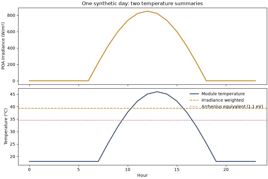
Daily in-plane irradiation: 6.46 kWh/m² (not an annual total)
Irradiance-weighted module temperature: 39.36 °C
Arrhenius-equivalent module temperature at 1.1 eV: 34.57 °C
Illustrative stress bin: T6:H4; no lifetime or degradation-rate prediction
import matplotlib.pyplot as plt
import numpy as np

from energy_methods.climate_zones import ClimateProvenance
from energy_methods.jrc_climate import performance_features
from energy_methods.pvcz import classify_pvcz, equivalent_temperature

hour = np.arange(24)
poa = 850 * np.maximum(0, np.sin((hour - 6) * np.pi / 12))
temperature = 18 + 28 * np.maximum(0, np.sin((hour - 7) * np.pi / 12))
energy, weighted = performance_features(poa, temperature)
teq = float(equivalent_temperature(temperature))
print(f"Daily in-plane irradiation: {energy:.2f} kWh/m² (not an annual total)")
print(f"Irradiance-weighted module temperature: {weighted:.2f} °C")
print(f"Arrhenius-equivalent module temperature at 1.1 eV: {teq:.2f} °C")
zone = classify_pvcz(
    teq,
    6,
    provenance=ClimateProvenance(
        "Synthetic daily cycle", "one illustrative day", "one site", "demonstration"
    ),
)
print(f"Illustrative stress bin: {zone.zone}; no lifetime or degradation-rate prediction")

fig, axes = plt.subplots(2, 1, figsize=(9, 6), sharex=True, layout="constrained")
axes[0].plot(hour, poa, color="#d18116", linewidth=2)
axes[0].set(ylabel="POA irradiance (W/m²)", title="One synthetic day: two temperature summaries")
axes[1].plot(hour, temperature, color="#324d70", label="Module temperature", linewidth=2)
axes[1].axhline(weighted, color="#d18116", linestyle="--", label="Irradiance weighted")
axes[1].axhline(teq, color="#b64152", linestyle=":", label="Arrhenius equivalent (1.1 eV)")
axes[1].set(xlabel="Hour", ylabel="Temperature (°C)")
axes[1].legend(frameon=False)
plt.show()
Total running time of the script: (0 minutes 0.117 seconds)