Note
Go to the end to download the full example code.
Bruna: Tenerife solar and wind forecast impact#
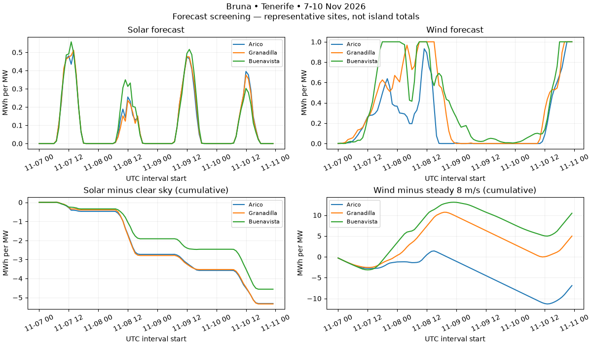
Frozen ECMWF IFS forecasts from Open-Meteo for 7-10 November 2026, retrieved before the event. This is a weather-to-power screening estimate, not measured production, causal storm attribution or a Tenerife fleet total. AEMET’s 6 November bulletin identified Bruna and forecast adverse weather in the Canary Islands.
Inputs are three representative coordinates, not a verified generator inventory. PV uses horizontal irradiance times 0.8 performance ratio; the solar reference is pvlib Ineichen clear sky at sea level. It is an upper-resource comparison, not normal November weather. Wind uses 120 m forecast speed with a generic cubic curve (3/12/25 m/s cut-in/rated/cut-out). A steady 8 m/s is the central assumed reference; 6 and 10 m/s show baseline sensitivity, not probability bounds.
All results are MWh per installed MW over 96 hours. No outages, storm damage, thermal generation, demand response, storage, wakes, terrain downscaling or curtailment are included. An island total requires plant capacities, locations, validated power curves and dispatch constraints. Gust warnings cannot be used as sustained hub-height speeds or proof of turbine shutdown.
Reproduce offline with uv run python examples/analysis/plot_bruna_tenerife.py.
The explicit acquisition step is uv run python scripts/prepare_bruna_forecast.py;
it refuses a new live run once the event starts, preventing hindsight leakage.
Frozen inputs and retrieval timestamps are in data/bruna.
One -1 W/m2 nighttime radiation value is clipped to zero; raw GHI is retained. Live API retrieval
time is not a model initialization timestamp. See Open-Meteo documentation for hourly radiation alignment and model details,
and pvlib clear-sky documentation
for the reference model. Weather data attribution: Open-Meteo / ECMWF, CC BY 4.0.
Forecast retrieval: 2026-11-06T23:55:16.948818+00:00
Per-MW screening; clear-sky solar and assumed wind references, NOT actual losses.
      site  baseline_wind_ms  pv_mwh_per_mw  pv_delta_mwh_per_mw  wind_mwh_per_mw  wind_delta_mwh_per_mw
     Arico               6.0          9.569               -5.314           20.463                  9.796
     Arico               8.0          9.569               -5.314           20.463                 -6.909
     Arico              10.0          9.569               -5.314           20.463                -34.450
Granadilla               6.0          9.559               -5.335           32.348                 21.682
Granadilla               8.0          9.559               -5.335           32.348                  4.976
Granadilla              10.0          9.559               -5.335           32.348                -22.565
Buenavista               6.0         10.294               -4.560           37.833                 27.166
Buenavista               8.0         10.294               -4.560           37.833                 10.461
Buenavista              10.0         10.294               -4.560           37.833                -17.080
import json
from pathlib import Path

import matplotlib.pyplot as plt
import pandas as pd

from energy_methods.storm_energy import storm_energy

example_dir = Path(__file__).resolve().parent if "__file__" in globals() else Path.cwd()
root = example_dir / "data" / "bruna"
weather = pd.read_csv(root / "bruna_forecast.csv", parse_dates=["timestamp"])
provenance = json.loads((root / "bruna_provenance.json").read_text())
print("Forecast retrieval:", provenance["records"][0]["retrieved_at_utc"])
print("Per-MW screening; clear-sky solar and assumed wind references, NOT actual losses.")
fig, axes = plt.subplots(2, 2, figsize=(12, 7), layout="constrained")
summary = []
for site, frame in weather.groupby("site", sort=False):
    result = storm_energy(frame)
    axes[0, 0].plot(result.timestamp, result.pv_mwh_per_mw, label=site)
    axes[0, 1].plot(result.timestamp, result.wind_mwh_per_mw, label=site)
    axes[1, 0].plot(result.timestamp, result.pv_delta_mwh_per_mw.cumsum(), label=site)
    axes[1, 1].plot(result.timestamp, result.wind_delta_mwh_per_mw.cumsum(), label=site)
    for baseline in (6.0, 8.0, 10.0):
        sensitivity = storm_energy(frame, baseline)
        summary.append(
            dict(
                site=site,
                baseline_wind_ms=baseline,
                pv_mwh_per_mw=result.pv_mwh_per_mw.sum(),
                pv_delta_mwh_per_mw=result.pv_delta_mwh_per_mw.sum(),
                wind_mwh_per_mw=result.wind_mwh_per_mw.sum(),
                wind_delta_mwh_per_mw=sensitivity.wind_delta_mwh_per_mw.sum(),
            )
        )
for ax, title in zip(
    axes.flat,
    [
        "Solar forecast",
        "Wind forecast",
        "Solar minus clear sky (cumulative)",
        "Wind minus steady 8 m/s (cumulative)",
    ],
    strict=True,
):
    ax.set(title=title, ylabel="MWh per MW", xlabel="UTC interval start")
    ax.tick_params(axis="x", rotation=25)
    ax.grid(alpha=0.2)
    ax.legend(fontsize=8)
fig.suptitle(
    "Bruna • Tenerife • 7-10 Nov 2026\nForecast screening — representative sites, not island totals"
)
print(pd.DataFrame(summary).round(3).to_string(index=False))
plt.show()
Total running time of the script: (0 minutes 0.356 seconds)