Note
Go to the end to download the full example code.
He Dreiht blade incident: shared versus independent wind-fleet risk#
News trigger (11 November 2026): Vestas’ Q3 earnings and Reuters coverage discuss costs after the July 2026 blade incident at EnBW’s He Dreiht offshore wind farm. The developer specified 64 Vestas V236-15 MW turbines, 960 MW total. Sources: https://www.vestas.com/en/investor/reports-and-presentations/vestas-reporting and https://www.offshorewind.biz/2026/08/12/all-turbines-installed-at-he-dreiht-offshore-wind-farm and https://www.reuters.com/business/energy/vestas-profit-hit-by-weak-volume-broken-turbine-blade-2026-11-11/
Business question: Can an independent-unit outage model understate the extreme energy exposure of a hypothetical shared fleet shutdown, even when both models have the same expected unavailable MW?
The 64 x 15 MW project nameplate is a published claim. ALL outage probabilities, shared-event assumptions, 24-hour duration, and capacity factor are SYNTHETIC, NOT OBSERVED. No blade defect frequency, fleet-wide failure, measured downtime, actual energy loss or warranty cost is inferred.
import matplotlib.pyplot as plt

from energy_methods.wind_shared_outage import screen_wind_shared_outage
Deliberately hypothetical 24-hour scenarios; not fitted to He Dreiht.
n = 64
rated_mw = 15.0
independent_p = 0.01
shared_q = 0.02
capacity_factor = 0.45
window_hours = 24.0

shared = screen_wind_shared_outage(
    turbine_count=n,
    rated_power_mw=rated_mw,
    independent_probability=independent_p,
    shared_event_probability=shared_q,
    shared_affected_turbines=n,
    capacity_factor=capacity_factor,
    window_hours=window_hours,
)

# Match the individual marginal probability, hence the expected unavailable MW.
p_marginal = shared_q + (1 - shared_q) * independent_p
independent = screen_wind_shared_outage(
    turbine_count=n,
    rated_power_mw=rated_mw,
    independent_probability=p_marginal,
    capacity_factor=capacity_factor,
    window_hours=window_hours,
)

assert abs(shared.expected_unavailable - independent.expected_unavailable) < 1e-10
for label, model in (
    ("Independent, mean-matched", independent),
    ("Shared-event scenario", shared),
):
    print(
        f"SYNTHETIC {label}: mean unavailable {model.expected_unavailable:.3f} "
        f"turbines; mean energy exposure {model.expected_exposure_mwh:.1f} MWh; "
        f"P(>=16 turbines unavailable)={model.at_least(16):.5%}; "
        f"P99 exposure={model.exposure_quantile_mwh(0.99):,.0f} MWh"
    )
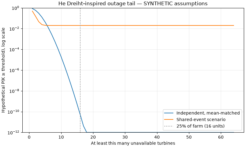
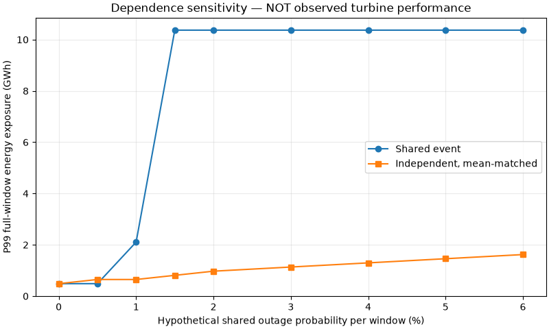
SYNTHETIC Independent, mean-matched: mean unavailable 1.907 turbines; mean energy exposure 309.0 MWh; P(>=16 turbines unavailable)=0.00000%; P99 exposure=972 MWh
SYNTHETIC Shared-event scenario: mean unavailable 1.907 turbines; mean energy exposure 309.0 MWh; P(>=16 turbines unavailable)=2.00000%; P99 exposure=10,368 MWh
Plot 1: at the same expected unavailability, dependence changes tail risk.
thresholds = range(1, n + 1)
fig, ax = plt.subplots(figsize=(8, 4.8), layout="constrained")
for label, model in (
    ("Independent, mean-matched", independent),
    ("Shared-event scenario", shared),
):
    ax.semilogy(
        list(thresholds),
        [max(model.at_least(k), 1e-12) for k in thresholds],
        label=label,
    )
ax.axvline(16, color="grey", linestyle=":", label="25% of farm (16 units)")
ax.set(
    xlabel="At least this many unavailable turbines",
    ylabel="Hypothetical P(K ≥ threshold), log scale",
    title="He Dreiht-inspired outage tail — SYNTHETIC assumptions",
    ylim=(1e-12, 1),
)
ax.legend()
ax.grid(alpha=0.25)
plt.show()
Plot 2: P99 24-hour energy-at-risk sensitivity to the assumed shared event.
shared_probabilities = [0, 0.005, 0.01, 0.015, 0.02, 0.03, 0.04, 0.05, 0.06]
scenario_p99 = []
mean_matched_p99 = []
for q in shared_probabilities:
    case = screen_wind_shared_outage(
        turbine_count=n,
        rated_power_mw=rated_mw,
        independent_probability=independent_p,
        shared_event_probability=q,
        shared_affected_turbines=n if q else 0,
        capacity_factor=capacity_factor,
        window_hours=window_hours,
    )
    counterfactual = screen_wind_shared_outage(
        turbine_count=n,
        rated_power_mw=rated_mw,
        independent_probability=q + (1 - q) * independent_p,
        capacity_factor=capacity_factor,
        window_hours=window_hours,
    )
    scenario_p99.append(case.exposure_quantile_mwh(0.99) / 1000)
    mean_matched_p99.append(counterfactual.exposure_quantile_mwh(0.99) / 1000)

fig, ax = plt.subplots(figsize=(8, 4.8), layout="constrained")
ax.plot(
    [100 * q for q in shared_probabilities],
    scenario_p99,
    marker="o",
    label="Shared event",
)
ax.plot(
    [100 * q for q in shared_probabilities],
    mean_matched_p99,
    marker="s",
    label="Independent, mean-matched",
)
ax.set(
    xlabel="Hypothetical shared outage probability per window (%)",
    ylabel="P99 full-window energy exposure (GWh)",
    title="Dependence sensitivity — NOT observed turbine performance",
)
ax.legend()
ax.grid(alpha=0.25)
plt.show()
Reproduce: uv run –no-sync python examples/analysis/plot_vestas_he_dreiht_blade_risk.py This example does not assess structural safety or operational decision rules.
Total running time of the script: (0 minutes 0.199 seconds)