Note
Go to the end to download the full example code.
Typical daily profiles#
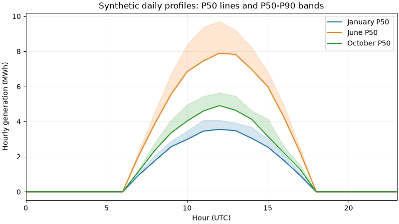
Compute monthly hourly P50/P90 profiles from synthetic generation. Here P90 is the empirical 90th percentile of hourly observations, not a 90% annual-energy exceedance estimate. Nighttime zeros remain observations.
import matplotlib.pyplot as plt
import numpy as np
import pandas as pd

from energy_methods.tdp import TDPConfig, analyze_tdp

timestamps = pd.date_range("2020-01-01", "2021-01-01", freq="h", inclusive="left", tz="UTC")
hours = timestamps.hour.to_numpy()
daylight = np.maximum(np.sin(np.pi * (hours - 6) / 12), 0)
season = 0.7 + 0.3 * np.cos(2 * np.pi * (timestamps.dayofyear.to_numpy() - 172) / 366)
rng = np.random.default_rng(42)
frame = pd.DataFrame(
    {
        "site_id": "synthetic_site",
        "timestamp": timestamps,
        "actual_mwh": 10 * daylight * season * rng.uniform(0.65, 1.0, len(timestamps)),
    }
)
# This generated signal has no measured solar-elevation evidence; explicitly
# disable positive-flat screening instead of inventing that input.
result = analyze_tdp(frame, TDPConfig(screen_positive_flat=False))

fig, ax = plt.subplots(figsize=(8, 4.5), layout="constrained")
for month, name in ((1, "January"), (6, "June"), (10, "October")):
    profile = result.avg.loc[result.avg["month"] == month]
    (line,) = ax.plot(profile["hour"], profile["p50"], label=f"{name} P50")
    ax.fill_between(
        profile["hour"], profile["p50"], profile["p90"], color=line.get_color(), alpha=0.18
    )
ax.set(
    xlabel="Hour (UTC)",
    ylabel="Hourly generation (MWh)",
    title="Synthetic daily profiles: P50 lines and P50-P90 bands",
    xlim=(0, 23),
)
ax.grid(alpha=0.2)
ax.legend()
plt.show()
Total running time of the script: (0 minutes 0.122 seconds)