Note
Go to the end to download the full example code.
Offshore wind transmission: quantify hypothetical cable outage exposure#
News (4 November 2026): Damage during installation of two Norderney export cables for Germany’s DolWin4 and BorWin4 links was reported. Amprion expects neither a material programme delay nor operational generation loss; the links are expected from 2028. The 1.8 GW combined link capacity is documented by Amprion, but not the capacity affected by either individual cable incident.
Sources: Tagesschau (4 November 2026), Amprion DolWin4/BorWin4 project overview, and DNV cable-repair context. Full dated links and provenance are provided in the method guide.
Business question: How much additional wind energy could go undelivered under hypothetical future export-cable outages, and how does it depend on repair duration, outage season and spare transmission capacity?
Evidence boundaries: All 400 days of input generation are SYNTHETIC, with an explicitly assumed 900-MW system, 900-MW export limit, and an illustrative 80 EUR/MWh realized energy price. Neither the 900-MW split nor prices nor weather are observed or attributed to either German link. The 60-day stress case is informed by a DNV repair-time reference, not a probability forecast. No outage loss is assigned to the 2026 construction accidents.
import math

import matplotlib.pyplot as plt

from energy_methods.offshore_cable_exposure import calculate_cable_exposure
Source-attributed context: Amprion reports 1.8 GW combined planned transfer. Engineering scenario only: one hypothetical 900-MW wind/export system. The 900 MW is NOT a verified capacity split of DolWin4 or BorWin4.
capacity_mw = 900.0
intervals = 400 * 24
hours = range(intervals)
wind_mw = [
    capacity_mw
    * min(
        1.0,
        max(
            0.0,
            0.46
            + 0.19 * math.sin(2 * math.pi * h / (24 * 11))
            + 0.11 * math.cos(2 * math.pi * h / (24 * 37))
            + 0.08 * math.cos(2 * math.pi * h / (24 * 365)),
        ),
    )
    for h in hours
]
# The deterministic waveform mimics resource variation, but is not calibrated
# to any wind plant, region, turbine power curve or measured weather record.
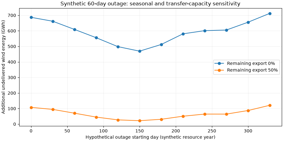
Energy accounting for a 60-day hypothetical future outage, day 120. DNV reports ~60 days as an industry-context export-cable repair duration. This is not an event rate, confidence interval, or expected outage duration.
case = calculate_cable_exposure(
    wind_mw,
    export_capacity_mw=capacity_mw,
    outage_start_interval=120 * 24,
    outage_intervals=60 * 24,
    outage_export_capacity_mw=0.0,
)
no_outage = calculate_cable_exposure(
    wind_mw,
    export_capacity_mw=capacity_mw,
    outage_start_interval=0,
    outage_intervals=0,
    outage_export_capacity_mw=0.0,
)
assert no_outage.incremental_lost_export_mwh == 0.0
assert math.isclose(
    case.incremental_lost_export_mwh,
    case.outage_curtailed_mwh - case.baseline_curtailed_mwh,
    abs_tol=1e-6,
)
print(f"SYNTHETIC reference wind exported: {no_outage.baseline_export_mwh:,.0f} MWh")
print(f"SYNTHETIC 60-day full-outage exposure: {case.incremental_lost_export_mwh:,.0f} MWh")
illustrative_price_eur_per_mwh = 80.0
print(
    "SYNTHETIC energy-value exposure (NOT realized loss): "
    f"EUR {case.incremental_lost_export_mwh * illustrative_price_eur_per_mwh / 1e6:.1f}m"
)
SYNTHETIC reference wind exported: 4,030,166 MWh
SYNTHETIC 60-day full-outage exposure: 498,285 MWh
SYNTHETIC energy-value exposure (NOT realized loss): EUR 39.9m
Sensitivity: outage season, 60 days, full vs half remaining export capacity.
starts_days = list(range(0, 331, 30))
fig, ax = plt.subplots(figsize=(9, 4.5), layout="constrained")
for remaining_fraction in (0.0, 0.5):
    exposures_gwh = [
        calculate_cable_exposure(
            wind_mw,
            export_capacity_mw=capacity_mw,
            outage_start_interval=start * 24,
            outage_intervals=60 * 24,
            outage_export_capacity_mw=remaining_fraction * capacity_mw,
        ).incremental_lost_export_mwh
        / 1e3
        for start in starts_days
    ]
    ax.plot(
        starts_days,
        exposures_gwh,
        marker="o",
        label=f"Remaining export {remaining_fraction:.0%}",
    )
ax.set(
    xlabel="Hypothetical outage starting day (synthetic resource year)",
    ylabel="Additional undelivered wind energy (GWh)",
    title="Synthetic 60-day outage: seasonal and transfer-capacity sensitivity",
)
ax.grid(alpha=0.2)
ax.legend()
plt.show()
Sensitivity: duration and redundant transfer capacity, fixed day 120.
fig, ax = plt.subplots(figsize=(9, 4.5), layout="constrained")
for remaining_fraction in (0.0, 0.5):
    days = [0, 7, 14, 30, 60, 90]
    values_gwh = [
        calculate_cable_exposure(
            wind_mw,
            export_capacity_mw=capacity_mw,
            outage_start_interval=120 * 24,
            outage_intervals=duration * 24,
            outage_export_capacity_mw=remaining_fraction * capacity_mw,
        ).incremental_lost_export_mwh
        / 1e3
        for duration in days
    ]
    ax.plot(
        days,
        values_gwh,
        marker="o",
        label=f"Remaining export {remaining_fraction:.0%}",
    )
ax.set(
    xlabel="Hypothetical outage duration (days)",
    ylabel="Additional undelivered wind energy (GWh)",
    title="Synthetic export-cable repair-duration sensitivity",
)
ax.legend()
ax.grid(alpha=0.2)
plt.show()
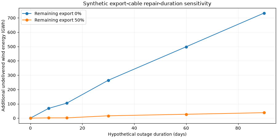
No failure frequency or probability is specified. The curves show deterministic what-if scenarios, NOT P10/P50/P90 risk or observed events. To reproduce: uv run –no-sync python examples/analysis/plot_norderney_cable_exposure.py
Total running time of the script: (0 minutes 0.224 seconds)