Note
Go to the end to download the full example code.
Solar and wind forecasting: four models, one common test#
Compare LightGBM, XGBoost, Mistral Timestral and physical surrogates with a previous-day baseline on real ONS plant observations. Each plant has 16 daily 24-hour forecasts after an initial 14-day training period. The default run fits the tree/physical models locally and replays checksum-verified real Timestral inference; it requires neither network access nor PyTorch.
Research inspiration: Ascencio-Vásquez, J., Bevc, J., Reba, K., Brecl, K., Jankovec, M. and Topič, M. (2020), Advanced PV Performance Modelling Based on Different Levels of Irradiance Data Accuracy, Energies 13(9), 2166. doi:10.3390/en13092166. Its attention to irradiance quality and empirical/ML comparisons motivates this example. This is a forecasting extension to different data, models and wind generation, not a reproduction of the paper’s experiment, accuracy tiers or numerical results.
Download the runnable example and data,
scores and
input provenance.
See the benchmark guide for model
equations, reproduction commands and methodological differences from the paper.
Scope: one solar plant and one wind farm in June 2024. Future weather is constructed by persistence, not archived NWP. Historical ONS data include post-operation revisions. Installed equipment and irradiance-plane metadata are incomplete; the physical models are explicit approximations. No universal model ranking or operational forecast claim follows from this small study.
1. Run the same chronological experiment for every model#
A forecast sees only the preceding 672 half-hour observations. Tree models share resource, clock sine/cosine and previous-day power features. Timestral receives the same covariates plus the full generation context. Physical surrogates use the resource forecast. All are evaluated on the same 768 future labels per plant, including nights and restricted-generation intervals.
import json
import os
from pathlib import Path

import matplotlib.dates as mdates
import matplotlib.pyplot as plt

from energy_analysis.forecast_benchmark import (
    MODELS,
    TIMESTRAL_MANIFEST,
    benchmark_scores,
    run_forecast_benchmark,
)
from energy_methods.timestral import TimestralConnector

directory = (
    Path(globals().get("__file__", Path.cwd() / "plot_forecast_model_benchmark.py"))
    .resolve()
    .parent
    / "data/forecast"
)
manifest = json.loads((directory / TIMESTRAL_MANIFEST).read_text())
connector = None
if os.environ.get("ENERGY_FORECAST_TIMESTRAL_LIVE") == "1":
    connector = TimestralConnector(
        manifest["model_id"],
        revision=manifest["model_revision"],
        device=os.environ.get("ENERGY_TIMESTRAL_DEVICE", "cpu"),
        local_files_only=os.environ.get("ENERGY_TIMESTRAL_LOCAL_ONLY") == "1",
    )
print("Timestral mode:", "live inference" if connector else "saved real inference, offline replay")
print(f"Checkpoint: {manifest['model_id']} @ {manifest['model_revision']}")
predictions = run_forecast_benchmark(directory, connector=connector)
scores = benchmark_scores(predictions)
lead_scores = benchmark_scores(predictions, by_lead=True)
print(scores.round(3).to_string(index=False))
if output := os.environ.get("ENERGY_FORECAST_OUTPUT"):
    destination = Path(output)
    destination.mkdir(parents=True, exist_ok=True)
    predictions.to_csv(destination / "predictions.csv", index=False)
    scores.to_csv(destination / "scores.csv", index=False)
    lead_scores.to_csv(destination / "lead_scores.csv", index=False)
Timestral mode: saved real inference, offline replay
Checkpoint: mistralai/Timestral-5M @ bdd20cfc15a3fea0e4cb5ccef37f8d3ca7aa335f
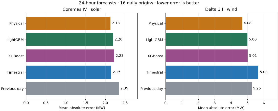
technology        model  samples  origins  mae_mw  rmse_mw  bias_mw  wape_pct  nmae_training_q95_pct  p10_p90_coverage  mae_skill_vs_previous_day
     solar     LightGBM      768       16   2.200    4.593   -0.010    38.131                 10.497               NaN                      0.063
     solar     Physical      768       16   2.133    4.190   -0.083    36.965                 10.163               NaN                      0.091
     solar Previous day      768       16   2.348    5.128    0.043    40.687                 11.216               NaN                      0.000
     solar    Timestral      768       16   2.152    4.271   -0.002    37.296                 10.261             0.637                      0.083
     solar      XGBoost      768       16   2.228    4.614    0.013    38.608                 10.629               NaN                      0.051
      wind     LightGBM      768       16   4.998    6.673   -0.019    71.348                 29.850               NaN                      0.049
      wind     Physical      768       16   4.683    6.120   -1.469    66.850                 27.975               NaN                      0.109
      wind Previous day      768       16   5.254    7.051    0.121    74.997                 31.233               NaN                      0.000
      wind    Timestral      768       16   5.663    7.413    1.030    80.836                 33.848             0.260                     -0.078
      wind      XGBoost      768       16   5.012    6.730    0.036    71.548                 29.941               NaN                      0.046
2. Compare errors without excluding difficult test observations#
MAE is in mean MW over a half-hour. RMSE, bias, WAPE, skill against the daily baseline and training-Q95-normalized MAE are printed above. The normalization uses historical power, not nameplate capacity, so it differs from the paper’s capacity-normalized RMSE. We do not apply its acceptance-band filtering or remove test outliers. Historical ONS resource flags mask model inputs only.
colors = dict(zip(MODELS, ("#c27619", "#287758", "#9a4d8b", "#2976b5", "#8b929b"), strict=True))
labels = {"solar": "Coremas IV · solar", "wind": "Delta 3 I · wind"}
fig, axes = plt.subplots(1, 2, figsize=(11, 4.4), layout="constrained")
for ax, technology in zip(axes, ("solar", "wind"), strict=True):
    table = scores[scores["technology"] == technology].set_index("model").loc[list(MODELS)]
    bars = ax.barh(table.index, table["mae_mw"], color=[colors[m] for m in table.index])
    ax.bar_label(bars, fmt="%.2f", padding=4)
    ax.invert_yaxis()
    ax.set(
        title=labels[technology],
        xlabel="Mean absolute error (MW)",
        xlim=(0, table["mae_mw"].max() * 1.2),
    )
    ax.grid(axis="x", alpha=0.2)
fig.suptitle("24-hour forecasts · 16 daily origins · lower error is better")
plt.show()
3. Inspect the final three days, chosen by date#
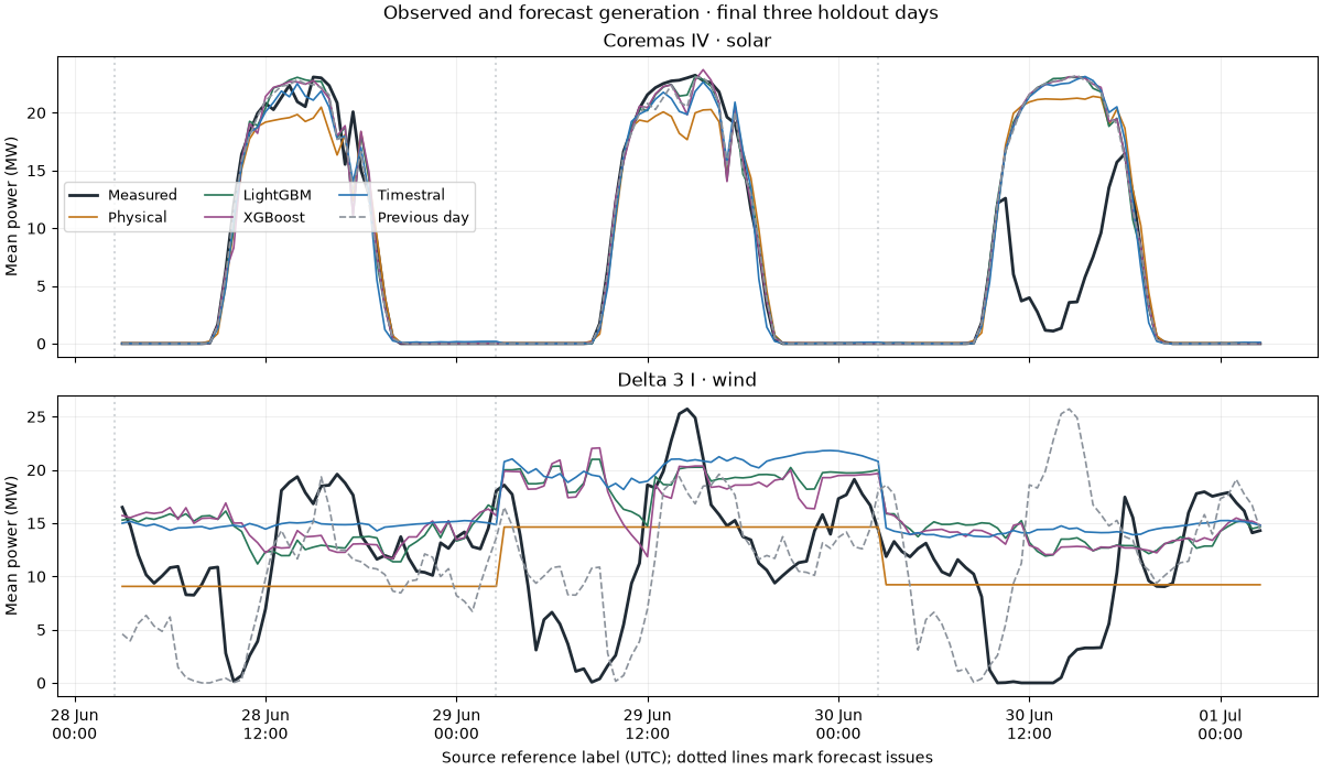
This fixed date slice is not selected for favorable errors. Daily model fits are concatenated here; forecasts are never updated within their 24-hour window.
fig, axes = plt.subplots(2, 1, figsize=(12, 7), layout="constrained", sharex=True)
for ax, technology in zip(axes, ("solar", "wind"), strict=True):
    case = predictions[predictions["technology"] == technology]
    last_issues = sorted(case["issue_time"].unique())[-3:]
    case = case[case["issue_time"].isin(last_issues)]
    actual = case[case["model"] == "Previous day"].sort_values("timestamp")
    ax.plot(
        actual["timestamp"], actual["actual_mw"], color="#202b35", linewidth=2, label="Measured"
    )
    for model in MODELS:
        rows = case[case["model"] == model].sort_values("timestamp")
        ax.plot(
            rows["timestamp"],
            rows["prediction_mw"],
            color=colors[model],
            label=model,
            linewidth=1.2,
            linestyle="--" if model == "Previous day" else "-",
        )
    for issue in last_issues:
        ax.axvline(issue, color="#abb2b9", alpha=0.5, linestyle=":")
    ax.set(title=labels[technology], ylabel="Mean power (MW)")
    ax.grid(alpha=0.2)
axes[0].legend(ncols=3, fontsize=9)
axes[-1].xaxis.set_major_formatter(mdates.DateFormatter("%d %b\n%H:%M"))
axes[-1].set_xlabel("Source reference label (UTC); dotted lines mark forecast issues")
fig.suptitle("Observed and forecast generation · final three holdout days")
plt.show()
4. Inspect error by forecast lead#
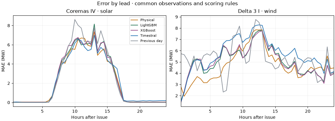
Each lead has 16 verification points per plant. Solar lead and clock time are coupled because every forecast is issued at the same daily clock time. These curves therefore reflect both horizon length and the daily resource cycle. Timestral P10-P90 coverage in the printed table is descriptive, not calibrated uncertainty. Pretraining overlap with this historical period is unknown.
fig, axes = plt.subplots(1, 2, figsize=(11, 4), layout="constrained")
for ax, technology in zip(axes, ("solar", "wind"), strict=True):
    for model in MODELS:
        rows = lead_scores[
            (lead_scores["technology"] == technology) & (lead_scores["model"] == model)
        ]
        ax.plot(rows["lead_hours"], rows["mae_mw"], color=colors[model], label=model)
    ax.set(title=labels[technology], xlabel="Hours after issue", ylabel="MAE (MW)", xlim=(0.5, 24))
    ax.grid(alpha=0.2)
axes[0].legend(fontsize=8)
fig.suptitle("Error by lead · common observations and scoring rules")
plt.show()
Total running time of the script: (0 minutes 2.291 seconds)