Note
Go to the end to download the full example code.
Taiwan: a real Taipower generation snapshot#
Read a complete genuine Taipower JSON publication with asset output, technology subtotals, status notes and storage-load rows. Values are MW snapshots. The ten-minute refresh cadence does not establish a ten-minute averaging interval, so this example does not integrate the values into energy.
The feed’s display labels can describe units, plants or groups. Known group labels and subtotals are distinguished from reported assets. Source: Taipower’s official open dataset, under Taiwan’s Open Government Data License 1.0.
Download the real JSON and
provenance alongside this
script in a data/ subdirectory. The example runs offline without a key.
import hashlib
import json
from pathlib import Path

import matplotlib.pyplot as plt

from energy_data_retrieval.sources.taipower import parse_generation
1. Verify and parse the original response#
directory = (
    Path(globals().get("__file__", Path.cwd() / "plot_generation_taipower.py")).resolve().parent
)
data = directory / "data"
raw = (data / "generation_taipower.json").read_bytes()
manifest = json.loads((data / "generation_taipower_provenance.json").read_text())
if hashlib.sha256(raw).hexdigest() != manifest["fixture_sha256"]:
    raise ValueError("Taipower sample differs from its acquisition manifest")
payload = json.loads(raw)
assets = parse_generation(payload)
complete = parse_generation(payload, include_aggregates=True, include_storage_load=True)
print("Publication time:", payload["DateTime"], "Asia/Taipei")
print("Default asset rows:", len(assets), "; all reported rows:", len(complete))
print(complete.groupby(["aggregation", "flow"]).size())
Publication time: 2026-10-30T16:00:00 Asia/Taipei
Default asset rows: 170 ; all reported rows: 213
aggregation       flow
reported_asset    consumption     10
                  generation     170
reported_group    consumption      1
                  generation      21
technology_total  generation      11
dtype: int64
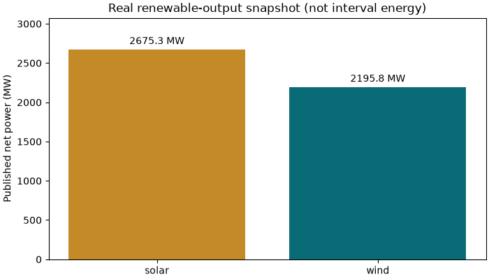
2. Plot the provider’s renewable subtotals as subtotals#
We select exactly one published subtotal per technology. We never add its children to the subtotal, which would double-count the same generation.
totals = complete.loc[complete.is_total & complete.technology.isin(["solar", "wind"])]
if len(totals) != 2:
    raise ValueError("The snapshot should have one solar and one wind subtotal")
fig, ax = plt.subplots(figsize=(7, 4), layout="constrained")
bars = ax.bar(totals.technology, totals.value, color=["#c48a28", "#096b76"])
ax.bar_label(bars, fmt="%.1f MW", padding=3)
ax.set(
    ylabel="Published net power (MW)", title="Real renewable-output snapshot (not interval energy)"
)
ax.margins(y=0.15)
plt.show()
3. Inspect individually reported assets and keep status notes#
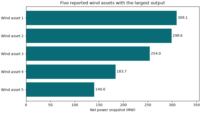
The plot uses numbered labels to avoid requiring a Chinese font. The printed table provides the exact original names and operating-status notes.
selected = assets.loc[assets.technology.eq("wind") & assets.value.notna()].nlargest(5, "value")
print(selected[["asset_id", "value", "capacity_mw", "source_status"]].to_string(index=False))
fig, ax = plt.subplots(figsize=(8, 4.5), layout="constrained")
labels = [f"Wind asset {index}" for index in range(1, len(selected) + 1)]
bars = ax.barh(labels, selected.value, color="#096b76")
ax.bar_label(bars, fmt="%.1f", padding=3)
ax.set(xlabel="Net power snapshot (MW)", title="Five reported wind assets with the largest output")
ax.invert_yaxis()
ax.margins(x=0.15)
plt.show()
asset_id  value  capacity_mw source_status
     沃一風  309.1        605.2
     海能風  298.6        376.0
沃四風(註10)  254.0          NaN
     芳二風  183.7        499.2
      允西  140.0        320.0
Total running time of the script: (0 minutes 0.137 seconds)