Note
Go to the end to download the full example code.
Spain: real generation by technology from REE#
This example reads actual public REData generation observations for June 2024. The complete API response is preserved with its retrieval time, source last-update metadata and SHA-256. The documentation build runs offline.
These are national totals by technology, not individual plant measurements. Values in the API are energy in MWh; charts below explicitly convert to GWh. Daily totals are not instantaneous power. See the generation connector guide for the other providers, access requirements and timestamp conventions.
Source: Red Eléctrica REData.
Download the real response,
provenance manifest, or
all generation examples with their data.
1. Retrieve a new snapshot when running your own analysis#
The public API needs no key. Use inclusive provider calendar dates. This example command requests one month without relying on the gallery snapshot:
uv run energy-retrieve ree-generation \
  --start 2024-06-01 --end 2024-06-30 --system national \
  --output data/ree_june_2024.parquet
Equivalent Python retrieval (shown but not called by the documentation):
from datetime import date
from energy_data_retrieval.transport import HTTPClient
from energy_data_retrieval.sources.ree import REE_HOSTS, REEClient
with HTTPClient(REE_HOSTS) as http:
    result = REEClient(http).generation(date(2024, 6, 1), date(2024, 6, 30))
observations, provenance = result.frame, result.requests
2. Verify and normalize the preserved real response#
The source’s Generación total rows are excluded by default. Including
them in a technology sum would count generation twice. Null observations
remain missing; absent technologies or dates are never filled with zero.
import hashlib
import json
from pathlib import Path

import matplotlib.pyplot as plt
import pandas as pd

from energy_data_retrieval.sources.ree import normalize_generation

example_directory = (
    Path(globals().get("__file__", Path.cwd() / "plot_generation_ree.py")).resolve().parent
)
data_dir = example_directory / "data"
sample_path = data_dir / "generation_ree.json"
manifest = json.loads((data_dir / "generation_ree_provenance.json").read_text())
raw = sample_path.read_bytes()
if hashlib.sha256(raw).hexdigest() != manifest["fixture_sha256"]:
    raise ValueError("The REE sample differs from its provenance manifest")
generation = normalize_generation(json.loads(raw))
print(
    f"Source: Red Eléctrica REData | {len(generation)} technology-period rows | "
    f"{generation['period'].nunique()} source calendar dates"
)
print("Retrieved:", manifest["request"]["retrieved_at_utc"])
print("Latest source update:", generation["source_last_update"].max())
print(generation[["timestamp", "technology", "value", "unit"]].head().to_string(index=False))
Source: Red Eléctrica REData | 451 technology-period rows | 30 source calendar dates
Retrieved: 2026-10-30T06:52:43.015058+00:00
Latest source update: 2026-01-13T17:55:06.000+01:00
                timestamp       technology      value unit
2024-05-31 22:00:00+00:00       Hidráulica  55208.696  MWh
2024-05-31 22:00:00+00:00           Carbón   7852.777  MWh
2024-05-31 22:00:00+00:00           Eólica 260654.250  MWh
2024-05-31 22:00:00+00:00 Otras renovables  10142.149  MWh
2024-05-31 22:00:00+00:00     Cogeneración  26020.593  MWh
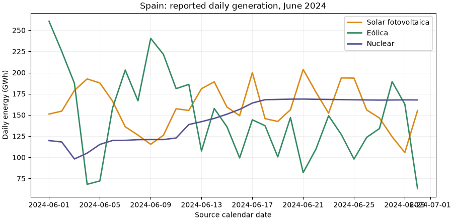
3. Compare daily wind, PV and nuclear energy#
period retains the source’s local calendar date, whereas timestamp
is its period-start label converted to UTC. Plot calendar dates when comparing
civil-day energy. Wind and PV are separate technologies; solar thermal is not PV.
daily = generation.pivot(index="period", columns="technology", values="value")
dates = pd.to_datetime(daily.index)
fig, ax = plt.subplots(figsize=(9, 4.4), layout="constrained")
for technology, color in [
    ("Solar fotovoltaica", "#db8a16"),
    ("Eólica", "#348b64"),
    ("Nuclear", "#555393"),
]:
    ax.plot(dates, daily[technology] / 1000, label=technology, color=color, linewidth=2)
ax.set(
    title="Spain: reported daily generation, June 2024",
    xlabel="Source calendar date",
    ylabel="Daily energy (GWh)",
)
ax.grid(alpha=0.2)
ax.legend()
plt.show()
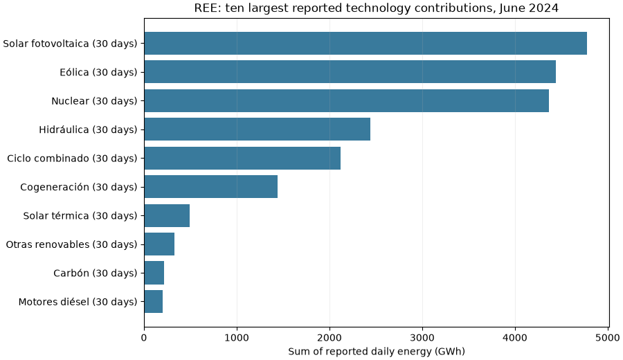
4. Inspect the month’s reported technology contributions#
Sum only the observations actually returned. Keep a count alongside each energy sum: a partial technology series does not establish complete coverage. This chart uses reported values, with no gap filling or extrapolation.
summary = generation.groupby("technology").agg(
    reported_mwh=("value", lambda values: values.sum(min_count=1)),
    reported_days=("value", "count"),
)
summary = summary.sort_values("reported_mwh").tail(10)
fig, ax = plt.subplots(figsize=(9, 5.2), layout="constrained")
labels = [f"{name} ({int(row.reported_days)} days)" for name, row in summary.iterrows()]
ax.barh(labels, summary["reported_mwh"] / 1000, color="#397a9c")
ax.set(
    title="REE: ten largest reported technology contributions, June 2024",
    xlabel="Sum of reported daily energy (GWh)",
)
ax.grid(axis="x", alpha=0.2)
plt.show()
Interpretation and scope#
REE may revise these historical data; the displayed source update is separate from our retrieval time. REData’s generation page states that this product excludes total estimated self-consumption, while including specified surplus injections. It cannot establish plant availability, capacity factor or a site’s production without separate plant and capacity evidence. Provider reuse terms apply to the preserved source data.
Total running time of the script: (0 minutes 0.205 seconds)