Note
Go to the end to download the full example code.
PV operation, failures and replacements through year 50#
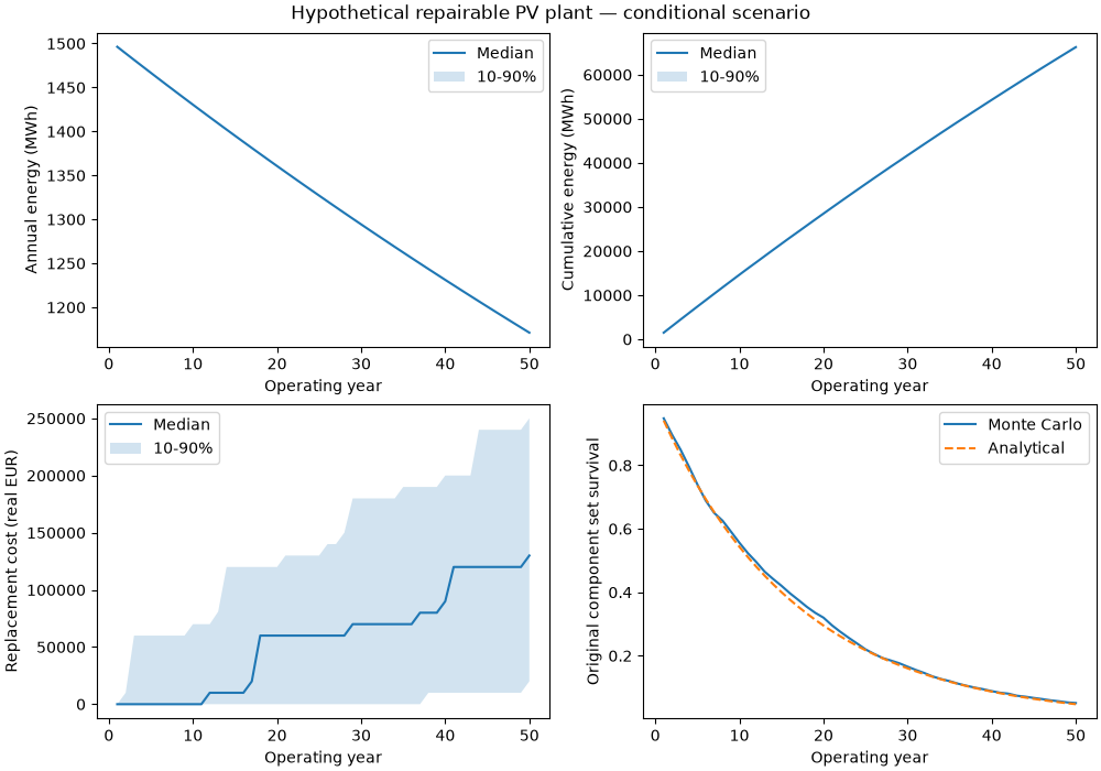
This offline engineering scenario extends the power-retention study with repairable component failures. All numerical inputs below are hypothetical. The 10th-90th percentile band represents sampled failures only, conditional on fixed inputs. It excludes degradation-parameter and weather uncertainty.
The model assumes at most one failure per component per year, independent annual probabilities and additive outage fractions capped at a full year. Replacing inverters restores service without rejuvenating the PV modules. Costs are constant-real illustrative EUR, without discounting or escalation.
import matplotlib.pyplot as plt

from energy_methods.pv_operation import ComponentScenario, simulate_operation
from energy_methods.pv_reliability import ReliabilityCurve

results = simulate_operation(
    curve=ReliabilityCurve("exponential", k=0.005),
    initial_annual_energy_mwh=1500,
    components=(
        ComponentScenario("inverter", 0.04, 14 / 365, 60_000),
        ComponentScenario("balance_of_system", 0.02, 7 / 365, 10_000),
    ),
    years=50,
    trials=2000,
    seed=42,
)

fig, axes = plt.subplots(2, 2, figsize=(10, 7), constrained_layout=True)
for ax, column, label in zip(
    axes.flat[:3],
    ["energy_mwh", "cumulative_energy_mwh", "cumulative_replacement_cost"],
    ["Annual energy (MWh)", "Cumulative energy (MWh)", "Replacement cost (real EUR)"],
    strict=True,
):
    bands = results.groupby("year")[column].quantile([0.1, 0.5, 0.9]).unstack()
    ax.plot(bands.index, bands[0.5], label="Median")
    ax.fill_between(bands.index, bands[0.1], bands[0.9], alpha=0.2, label="10-90%")
    ax.set(xlabel="Operating year", ylabel=label)
    ax.legend()
survival = results.groupby("year")["original_components_survive"].mean()
axes[1, 1].plot(survival.index, survival, label="Monte Carlo")
axes[1, 1].plot(survival.index, (0.96 * 0.98) ** survival.index, "--", label="Analytical")
axes[1, 1].set(xlabel="Operating year", ylabel="Original component set survival")
axes[1, 1].legend()
fig.suptitle("Hypothetical repairable PV plant — conditional scenario")
plt.show()
Compare operating horizons#
Each horizon uses the same simulated histories, avoiding independent resampling.
print(
    results[results.year.isin([30, 40, 50])]
    .groupby("year")[["cumulative_energy_mwh", "cumulative_replacement_cost"]]
    .mean()
    .to_string()
)
# Optional export after running this downloaded example:
# results.to_csv("pv_operation_trials.csv", index=False)
      cumulative_energy_mwh  cumulative_replacement_cost
year
30             41707.012841                      78920.0
40             54275.905915                     104710.0
50             66231.444739                     131345.0
Total running time of the script: (0 minutes 0.241 seconds)