Note
Go to the end to download the full example code.
Chile curtailment and equivalent storage: reproduce the published findings#
Acosta et al., Journal of Energy Storage 183 (2027), 125203, online October 2026. DOI: https://doi.org/10.1016/j.est.2026.125203.
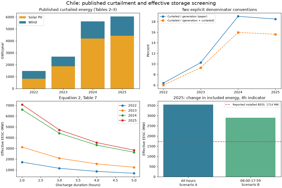
Business question: How large is Chile’s reported curtailment exposure, and how does the paper’s equivalent-storage indicator change with duration and daytime-only scope? Published aggregates are reproduced offline, with rounding audits. These are not a fresh CEN download or a feasible battery design.
The paper’s 18.49% divides curtailment by reported generation. We also show the
potential-energy denominator. Hourly exports can be analyzed separately using
python -m energy_analysis.chile_curtailment --hourly-config config.json;
see docs/chile-curtailment-storage.md for the source contract and limitations.
import matplotlib.pyplot as plt

from energy_analysis.chile_curtailment import reproduce_published_tables

results = reproduce_published_tables()
assert results["audit"]["matches_expected_agreement"].all(), "Unexpected published-table agreement"
annual = results["annual"]
scenarios = results["scenarios"].iloc[0]
print(annual.to_string(index=False))
print(f"Published comparisons within tolerance: {results['audit']['within_tolerance'].sum()}/35")
print("Source discrepancy: 2024 total computes to 19.0009%, versus 18.99% in Table 3.")
print(f"2025 effective 4h indicator: {scenarios['scenario_a_mw']:.1f} MW")
print(f"Uncovered indicator after 1714 MW installed BESS: {scenarios['uncovered_a_mw']:.1f} MW")
print(
    f"Block B only: {scenarios['scenario_b_mw']:.1f} MW; "
    f"reduction: {scenarios['reduction_relative_to_a_pct']:.2f}%"
)
 year  pv_curtailment_gwh  wind_curtailment_gwh  total_curtailment_gwh  generation_gwh  curtailed_over_generated_pct  curtailed_over_potential_pct  eesc_4h_mw  installed_bess_mw  uncovered_4h_mw
 2022               829.9                 641.1                 1471.0           23047                      6.382609                      5.999674  861.441781                  0       861.441781
 2023              1862.2                 804.4                 2666.6           25986                     10.261679                      9.306660 1561.604795                179      1382.604795
 2024              4189.5                1453.0                 5642.5           29696                     19.000876                     15.967005 3304.340753                861      2443.340753
 2025              4424.3                1619.8                 6044.1           32685                     18.491969                     15.606095 3539.524315               1714      1825.524315
Published comparisons within tolerance: 34/35
Source discrepancy: 2024 total computes to 19.0009%, versus 18.99% in Table 3.
2025 effective 4h indicator: 3539.5 MW
Uncovered indicator after 1714 MW installed BESS: 1825.5 MW
Block B only: 2900.9 MW; reduction: 18.04%
Annual source figures and the two denominators must be interpreted separately.
fig, axes = plt.subplots(2, 2, figsize=(12, 8), layout="constrained")
fig.suptitle("Chile: published curtailment and effective storage screening", fontsize=15)
years = annual["year"].astype(str)
axes[0, 0].bar(years, annual["pv_curtailment_gwh"], label="Solar PV", color="#e8a225")
axes[0, 0].bar(
    years,
    annual["wind_curtailment_gwh"],
    bottom=annual["pv_curtailment_gwh"],
    label="Wind",
    color="#357f9a",
)
axes[0, 0].set(title="Published curtailed energy (Tables 2-3)", ylabel="GWh/year")
axes[0, 0].legend()
axes[0, 1].plot(
    years, annual["curtailed_over_generated_pct"], "o-", label="Curtailed / generation (paper)"
)
axes[0, 1].plot(
    years,
    annual["curtailed_over_potential_pct"],
    "s--",
    label="Curtailed / (generation + curtailed)",
)
axes[0, 1].set(title="Two explicit denominator conventions", ylabel="Percent")
axes[0, 1].legend(fontsize=8)
for year, group in results["duration"].groupby("year"):
    axes[1, 0].plot(group["duration_hours"], group["eesc_mw"], "o-", label=str(year))
axes[1, 0].set(
    title="Equation 2, Table 7", xlabel="Discharge duration (hours)", ylabel="Effective EESC (MW)"
)
axes[1, 0].legend()
axes[1, 1].bar(
    ["All hours\nScenario A", "08:00-17:59\nScenario B"],
    [scenarios["scenario_a_mw"], scenarios["scenario_b_mw"]],
    color=["#357f9a", "#5eaf8b"],
)
axes[1, 1].axhline(1714, color="#b44b42", linestyle="--", label="Reported installed BESS: 1714 MW")
axes[1, 1].set(title="2025: change in included energy, 4h indicator", ylabel="Effective EESC (MW)")
axes[1, 1].legend(fontsize=8)
plt.show()
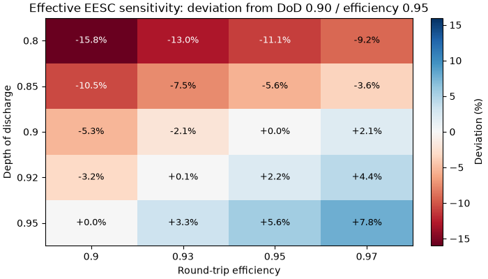
The sensitivity retains the paper’s multiplication by DoD and efficiency. Lower efficiency lowers this effective indicator, not required nameplate size.
matrix = (
    results["sensitivity"]
    .query("duration_hours == 4")
    .pivot(
        index="depth_of_discharge",
        columns="round_trip_efficiency",
        values="deviation_from_baseline_pct",
    )
)
fig, ax = plt.subplots(figsize=(7, 4), layout="constrained")
heat = ax.imshow(matrix.to_numpy(), cmap="RdBu", aspect="auto", vmin=-16, vmax=16)
ax.set(
    xticks=range(len(matrix.columns)),
    xticklabels=matrix.columns,
    yticks=range(len(matrix.index)),
    yticklabels=matrix.index,
    xlabel="Round-trip efficiency",
    ylabel="Depth of discharge",
    title="Effective EESC sensitivity: deviation from DoD 0.90 / efficiency 0.95",
)
for row in range(len(matrix.index)):
    for col in range(len(matrix.columns)):
        ax.text(
            col,
            row,
            f"{matrix.iloc[row, col]:+.1f}%",
            ha="center",
            va="center",
            fontsize=9,
            color="white" if abs(matrix.iloc[row, col]) > 10 else "black",
        )
fig.colorbar(heat, ax=ax, label="Deviation (%)")
plt.show()
Total running time of the script: (0 minutes 0.381 seconds)