Note
Go to the end to download the full example code.
Germany: onshore wind permitting-to-grid capacity bottlenecks#
News trigger: Reuters, 6 November 2026, reported German onshore wind transport delays and grid connection constraints despite record approvals. https://www.reuters.com/business/energy/germanys-onshore-wind-boom-faces-logistical-hurdles-turbine-orders-surge-2026-11-06/
Business question: For already-approved onshore wind projects, which annual throughput expansion unlocks commissioning: transport, erection or grid?
Observed published aggregates (not individual project time series): German industry/Fachagentur Wind und Solar reported 48.1 GW approved but not operating as of 30 June 2026, with about 19 GW still without auction awards. Sources and caveats: onshore logistics scenario guide.
ILLUSTRATIVE hypothetical assumptions: annual transport, erection, awards and grid throughput rates; zero new approvals to isolate that historical cohort. This is NOT a 2027-2032 forecast. See the documentation for provenance and boundary conditions. Runs offline and uses no downloaded copyrighted tables.
Published sources anchor the size of the approved cohort only.
import matplotlib.pyplot as plt
import numpy as np

from energy_methods.wind_pipeline import simulate_wind_pipeline

SOURCE_PIPELINE_GW = 48.1
SOURCE_UNAWARDED_GW = 19.0
SOURCE_AS_OF = "2026-06-30"
SYNTHETIC_YEARS = tuple(range(2027, 2033))


def scenario(*, transport_gw: float, grid_gw: float):
    """Hypothetical annual throughput scenario, not calibrated to Germany."""
    return simulate_wind_pipeline(
        first_year=SYNTHETIC_YEARS[0],
        initial_unawarded_gw=SOURCE_UNAWARDED_GW,
        initial_awarded_gw=SOURCE_PIPELINE_GW - SOURCE_UNAWARDED_GW,
        new_approvals_gw=(0.0,) * len(SYNTHETIC_YEARS),
        awards_per_year_gw=15.0,  # invented scenario, not 2027 auction realization
        transport_per_year_gw=transport_gw,
        erection_per_year_gw=12.0,
        grid_per_year_gw=grid_gw,
    )
Paired sensitivity: changes only in transport and/or grid throughput.
cases = {
    "Baseline: 6 GW transport / 7 GW grid": scenario(transport_gw=6, grid_gw=7),
    "Transport expansion: 11 / 7": scenario(transport_gw=11, grid_gw=7),
    "Grid expansion: 6 / 12": scenario(transport_gw=6, grid_gw=12),
    "Both expansions: 11 / 12": scenario(transport_gw=11, grid_gw=12),
}

for name, values in cases.items():
    end = values[-1]
    print(
        f"SYNTHETIC {name}: commissioned={end.cumulative_commissioned_gw:.1f} GW, "
        f"awaiting award={end.waiting_for_award_gw:.1f} GW, "
        f"awaiting transport={end.waiting_for_transport_gw:.1f} GW, "
        f"awaiting erection={end.waiting_for_erection_gw:.1f} GW, "
        f"awaiting grid={end.waiting_for_grid_gw:.1f} GW"
    )

fig, ax = plt.subplots(figsize=(10, 5), layout="constrained")
for name, result in cases.items():
    ax.plot(
        SYNTHETIC_YEARS,
        [row.cumulative_commissioned_gw for row in result],
        marker="o",
        label=name,
    )
ax.axhline(SOURCE_PIPELINE_GW, ls="--", color="gray", label="Published approved stock")
ax.set(
    title="Germany onshore: HYPOTHETICAL bottleneck capacity scenarios",
    xlabel="Illustrative calendar year (no project-level timing calibration)",
    ylabel="Cumulative commissioned GW from June 2026 cohort",
    ylim=(0, SOURCE_PIPELINE_GW * 1.12),
)
ax.legend(fontsize=8)
plt.show()
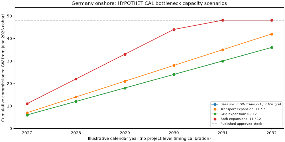
SYNTHETIC Baseline: 6 GW transport / 7 GW grid: commissioned=36.0 GW, awaiting award=0.0 GW, awaiting transport=12.1 GW, awaiting erection=0.0 GW, awaiting grid=0.0 GW
SYNTHETIC Transport expansion: 11 / 7: commissioned=42.0 GW, awaiting award=0.0 GW, awaiting transport=0.0 GW, awaiting erection=0.0 GW, awaiting grid=6.1 GW
SYNTHETIC Grid expansion: 6 / 12: commissioned=36.0 GW, awaiting award=0.0 GW, awaiting transport=12.1 GW, awaiting erection=0.0 GW, awaiting grid=0.0 GW
SYNTHETIC Both expansions: 11 / 12: commissioned=48.1 GW, awaiting award=0.0 GW, awaiting transport=0.0 GW, awaiting erection=0.0 GW, awaiting grid=0.0 GW
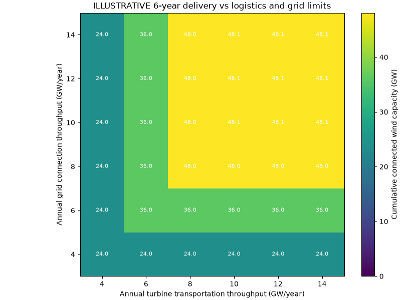
Two-dimensional bottleneck surface: a larger construction throughput alone cannot overcome a smaller capacity at another mandatory stage.
transport_values = np.array([4, 6, 8, 10, 12, 14], dtype=float)
grid_values = np.array([4, 6, 8, 10, 12, 14], dtype=float)
commissioned = np.array(
    [
        [
            scenario(transport_gw=float(t), grid_gw=float(g))[-1].cumulative_commissioned_gw
            for t in transport_values
        ]
        for g in grid_values
    ]
)
fig, ax = plt.subplots(figsize=(8, 6), layout="constrained")
heatmap = ax.imshow(commissioned, origin="lower", cmap="viridis", vmin=0, vmax=SOURCE_PIPELINE_GW)
ax.set_xticks(range(len(transport_values)), [str(int(t)) for t in transport_values])
ax.set_yticks(range(len(grid_values)), [str(int(g)) for g in grid_values])
ax.set(
    title="ILLUSTRATIVE 6-year delivery vs logistics and grid limits",
    xlabel="Annual turbine transportation throughput (GW/year)",
    ylabel="Annual grid connection throughput (GW/year)",
)
for row in range(len(grid_values)):
    for column in range(len(transport_values)):
        ax.text(
            column,
            row,
            f"{commissioned[row, column]:.1f}",
            ha="center",
            va="center",
            color="white",
            fontsize=8,
        )
fig.colorbar(heatmap, ax=ax, label="Cumulative connected wind capacity (GW)")
plt.show()
Model controls and limitations: optimistic within-year flow through stages, aggregated national stocks, no actual projects, weather, permits, cancellations, financing, location-specific access roads, line upgrades or energy output. 2025 annual approval/installation values are independent cohorts and MUST NOT be subtracted to infer project-level conversion times.
Total running time of the script: (0 minutes 0.227 seconds)