Note
Go to the end to download the full example code.
Ecowende: adaptive wind curtailment versus wildlife-activity exposure#
News (2 November 2026): Eneco reports that all 52 Ecowende turbines were installed by 30 October. The ~760 MW Dutch offshore project incorporates adaptive curtailment and AI-assisted radar monitoring for birds and bats.
Decision question: In an illustrative wind farm, how much renewable energy is retained by stopping turbines only in elevated-activity periods rather than blanket nighttime shutdown? Can a fractional energy-minimizing policy attain the same activity-exposure proxy reduction as a radar-triggered threshold?
Evidence: Eneco’s dated installation announcement: https://nieuws.eneco.nl/van-oord-en-vestas-plaatsen-laatste-windturbine-van-ecowende-windpark-gaat-de-afrondende-fase-van-de-constructie-in Waardenburg Ecology documents a real (other-site) radar threshold protocol: https://waardenburg.eco/en-gb/project/stopping-wind-turbines-3d-bird-radar
Data boundary: All hourly wind speeds and bird-activity indices below are SYNTHETIC. No Ecowende wind speeds, measured radar traffic, collisions, collision-avoidance effectiveness or field energy losses are available in this example. The proxy is not a bird-mortality model; no wildlife benefit or actual revenue is inferred. See the following documentation: method guide.
import math

import matplotlib.pyplot as plt

from energy_methods.wildlife_curtailment import (
    min_energy_loss_schedule,
    screen_wildlife_curtailment,
)
Synthetic deterministic 14-day profile. Approximate wind power curve: cubic below rated, zero below cut-in/above cut-out. Site and curve uncalibrated.
capacity_mw = 760.0  # Eneco reports APPROXIMATE project capacity, not metered output.
hours = range(14 * 24)
wind_speed_ms = [
    8.8 + 2.4 * math.sin(2 * math.pi * h / 48) + 1.5 * math.cos(2 * math.pi * h / 79) for h in hours
]


def illustrative_power_mw(speed_ms: float) -> float:
    """Synthetic power curve; no claim to represent a Vestas turbine."""
    if speed_ms < 3 or speed_ms >= 25:
        return 0.0
    if speed_ms >= 12:
        return capacity_mw
    return capacity_mw * (speed_ms**3 - 3**3) / (12**3 - 3**3)


power_mw = [illustrative_power_mw(speed) for speed in wind_speed_ms]
# Radar-like traffic INDICES, not actual measurements or calibrated risk scores.
activity = [
    (0.15 if 7 <= h % 24 < 18 else 0.8)
    + (4.0 if (h // 24) % 5 in (1, 2) and 19 <= h % 24 <= 23 else 0.0)
    + 0.25 * (1 + math.sin(2 * math.pi * h / 37))
    for h in hours
]
Three explicit strategies. Threshold is an illustrative detector trigger; blanket shutdown is a precautionary comparison, NOT an Ecowende policy.
no_shutdown = [0.0] * len(power_mw)
blanket_night = [1.0 if h % 24 >= 18 or h % 24 < 6 else 0.0 for h in hours]
radar_triggered = [1.0 if index >= 3.0 else 0.0 for index in activity]
no_action = screen_wildlife_curtailment(power_mw, activity, no_shutdown)
blanket = screen_wildlife_curtailment(power_mw, activity, blanket_night)
radar = screen_wildlife_curtailment(power_mw, activity, radar_triggered)
# Continuous interval optimization at the *same proxy* as the threshold case.
optimized = screen_wildlife_curtailment(
    power_mw,
    activity,
    min_energy_loss_schedule(power_mw, activity, radar.proxy_reduction_fraction),
)

for label, result in [
    ("No curtailment", no_action),
    ("Blanket night", blanket),
    ("Radar threshold", radar),
    ("Fractional proxy optimum", optimized),
]:
    print(
        f"SYNTHETIC {label:25s}: lost {result.curtailed_energy_mwh / 1000:.2f} GWh; "
        f"activity-index exposure reduction {result.proxy_reduction_fraction:.1%}"
    )
assert optimized.proxy_reduction_fraction >= radar.proxy_reduction_fraction - 1e-10
assert optimized.curtailed_energy_mwh <= radar.curtailed_energy_mwh + 1e-7
SYNTHETIC No curtailment           : lost 0.00 GWh; activity-index exposure reduction 0.0%
SYNTHETIC Blanket night            : lost 54.64 GWh; activity-index exposure reduction 79.5%
SYNTHETIC Radar threshold          : lost 10.35 GWh; activity-index exposure reduction 40.9%
SYNTHETIC Fractional proxy optimum : lost 9.41 GWh; activity-index exposure reduction 40.9%
Figure 1: explicit energy/exposure tradeoff (NOT mortality reduction).
labels = ["No action", "Night blanket", "Radar threshold", "Proxy optimum"]
results = [no_action, blanket, radar, optimized]
fig, ax = plt.subplots(figsize=(8, 4.5), layout="constrained")
for label, result in zip(labels, results, strict=True):
    ax.scatter(
        result.curtailed_energy_mwh / 1000,
        result.proxy_reduction_fraction * 100,
        s=90,
        label=label,
    )
ax.set(
    xlabel="Modeled generation curtailed over 14 days (GWh)",
    ylabel="Activity-weighted rotor-hours proxy removed (%)",
    title="Ecowende-inspired screening — SYNTHETIC, not collision avoidance",
)
ax.legend(loc="best")
ax.grid(alpha=0.2)
plt.show()
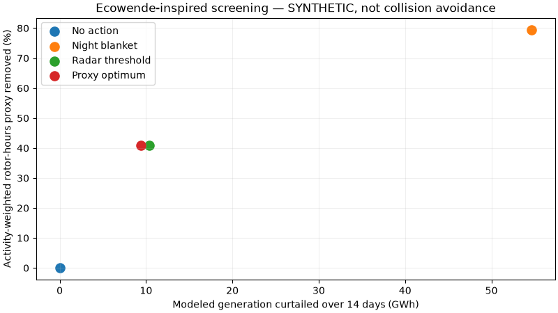
Figure 2: perfect-foresight bound for a range of proxy targets.
proxy_targets = [k / 20 for k in range(21)]
frontier = [
    screen_wildlife_curtailment(
        power_mw, activity, min_energy_loss_schedule(power_mw, activity, target)
    ).curtailed_energy_mwh
    / 1000
    for target in proxy_targets
]
fig, ax = plt.subplots(figsize=(8, 4.5), layout="constrained")
ax.plot([100 * t for t in proxy_targets], frontier, marker="o", label="Continuous LP bound")
ax.scatter(
    [100 * radar.proxy_reduction_fraction],
    [radar.curtailed_energy_mwh / 1000],
    marker="x",
    s=100,
    label="Illustrative threshold policy",
)
ax.set(
    xlabel="Target reduction in synthetic activity-exposure proxy (%)",
    ylabel="Minimum modeled curtailed energy (GWh / 14 days)",
    title="Theoretical minimum energy loss; perfect activity foresight assumed",
)
ax.legend()
ax.grid(alpha=0.2)
plt.show()
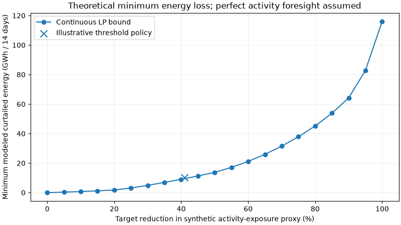
Do not extrapolate the 14-day profile to annual costs or wildlife mortality. The continuous optimum is NOT implementable as a live-control algorithm without forecasts, operational constraints, species validation and independent monitoring. Reproduce: uv run –no-sync python examples/analysis/plot_ecowende_wildlife_curtailment.py
Total running time of the script: (0 minutes 0.191 seconds)