Note
Go to the end to download the full example code.
Map KGPV climate zones worldwide#
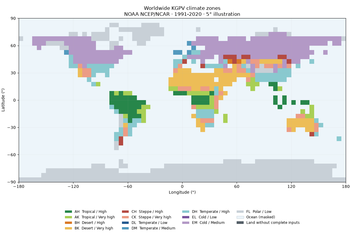
Classify real, gridded temperature, rainfall and solar climatologies with
energy_methods.kgpv.map_kgpv(), then plot the twelve KGPV zones and their
area distribution. The inputs are derived from NOAA PSL NCEP/NCAR Reanalysis 1,
1991-2020, sampled on a coarse 5° grid. Oceans are masked.
This is a reproducible illustration using an alternative climate source, not a reproduction of the original published KGPV map. The classification follows the repository’s fixed thresholds and twelve-zone merges. Coarse coastal cells and reanalysis biases affect zone boundaries and area estimates.
Download the input CSV and
provenance JSON alongside this script.
Run it with those files in the working directory; in a repository checkout:
uv sync --locked --all-packages --group docs
cd examples/analysis
uv run python plot_kgpv_worldwide.py
The example makes no network requests and needs no credentials or mapping downloads. See the KGPV guide for source preparation, unit conversions, citations and the GPCC/CRU workflow.
import hashlib
import json
from pathlib import Path

import matplotlib.pyplot as plt
import numpy as np
import pandas as pd
import xarray as xr
from matplotlib.colors import BoundaryNorm, ListedColormap
from matplotlib.patches import Patch

from energy_methods.kgpv import IRRADIATION_NAMES, TP_NAMES, ZONE_CODES, map_kgpv
from energy_methods.mapping import class_area_summary, write_geojson
Load the attributed climate inputs#
Check the CSV against its acquisition/preparation manifest. Blank values are
missing data; they must never become zero rainfall or zero irradiation.
t01…t12 are °C, p01…p12 are monthly mm, and annual_ghi is
kWh/m²/year. Every variable carries the same climatological baseline.
csv_path = Path("kgpv_worldwide_inputs.csv")
provenance = json.loads(Path("kgpv_worldwide_provenance.json").read_text(encoding="utf-8"))
if hashlib.sha256(csv_path.read_bytes()).hexdigest() != provenance["fixture_sha256"]:
    raise ValueError("Input fixture checksum differs from its provenance")
table = pd.read_csv(csv_path).set_index(["lat", "lon"]).to_xarray()
baseline = {key: provenance[key] for key in ("baseline_start_year", "baseline_end_year")}
months = xr.IndexVariable("month", np.arange(1, 13))
temperature = xr.concat([table[f"t{m:02d}"] for m in range(1, 13)], dim=months)
precipitation = xr.concat([table[f"p{m:02d}"] for m in range(1, 13)], dim=months)
annual_ghi = table.annual_ghi
for field, units in (
    (temperature, "degC"),
    (precipitation, "mm"),
    (annual_ghi, "kWh m-2"),
):
    field.attrs = {**baseline, "units": units, "source": provenance["source"]}
Classify continuous climate inputs#
The preparation script regrids the continuous variables before applying
thresholds. Categorical class IDs are never bilinearly interpolated.
map_kgpv checks units, coordinates and baseline consistency; incomplete
cells receive class 0. The CSV already masks ocean cells using NOAA’s land mask.
result = map_kgpv(temperature, precipitation, annual_ghi)
classes = result.kgpv_class
zones = ZONE_CODES[1:]
print(f"Baseline: {baseline['baseline_start_year']}-{baseline['baseline_end_year']}")
print(f"Classified land cells: {int((classes > 0).sum())} / {int(table.is_land.sum())}")
Baseline: 1991-2020
Classified land cells: 858 / 858
Draw the worldwide map#
A regular longitude/latitude view needs only Matplotlib. The legend includes all twelve merged zones even when one is absent in this coarse sample. Land without complete inputs is gray; masked ocean is pale blue. Coastal squares represent centre-sampled model cells, not precise coastlines.
colors = [
    "#27864a",
    "#a9cf55",  # tropical: AH, AK
    "#d97927",
    "#edbd57",  # desert: BH, BK
    "#b44a42",
    "#ec9c85",  # steppe: CH, CK
    "#265a90",
    "#5399be",
    "#89c9cf",  # temperate: DL, DM, DH
    "#79559d",
    "#b399c6",  # cold: EL, EM
    "#c8d0d7",  # polar: FL
]
cmap = ListedColormap(colors)
norm = BoundaryNorm(np.arange(0.5, 13.5), cmap.N)
lon_edges = np.arange(-180, 181, 5)
lat_edges = np.arange(-90, 91, 5)
ocean_color, missing_color = "#edf5fa", "#555f68"

fig = plt.figure(figsize=(12, 8.2), layout="constrained")
grid = fig.add_gridspec(2, 1, height_ratios=[6, 1.2])
ax = fig.add_subplot(grid[0])
legend_ax = fig.add_subplot(grid[1])
legend_ax.axis("off")
ax.set_facecolor(ocean_color)
ax.pcolormesh(
    lon_edges,
    lat_edges,
    np.ma.masked_where(table.is_land.values != 1, np.ones(classes.shape)),
    cmap=ListedColormap([missing_color]),
    shading="flat",
    rasterized=True,
)
ax.pcolormesh(
    lon_edges,
    lat_edges,
    np.ma.masked_equal(classes.values, 0),
    cmap=cmap,
    norm=norm,
    shading="flat",
    rasterized=True,
)
ax.set(
    xlim=(-180, 180),
    ylim=(-90, 90),
    aspect="equal",
    xticks=np.arange(-180, 181, 60),
    yticks=np.arange(-90, 91, 30),
    xlabel="Longitude (°)",
    ylabel="Latitude (°)",
    title="Worldwide KGPV climate zones\nNOAA NCEP/NCAR · 1991-2020 · 5° illustration",
)
ax.grid(alpha=0.15, linewidth=0.6)
handles = [
    Patch(facecolor=color, label=f"{zone}  {TP_NAMES[zone[0]]} / {IRRADIATION_NAMES[zone[1]]}")
    for zone, color in zip(zones, colors, strict=True)
]
handles += [
    Patch(facecolor=ocean_color, edgecolor="#ccd7df", label="Ocean (masked)"),
    Patch(facecolor=missing_color, label="Land without complete inputs"),
]
legend_ax.legend(
    handles=handles,
    loc="center",
    ncol=4,
    frameon=False,
    fontsize=8.5,
)
plt.show()
Summarize classified land area#
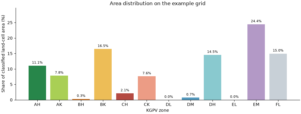
Use spherical cell areas, not equally weighted pixel counts: polar grid cells cover less area than equatorial cells. The denominator is classified land-cell area, excluding ocean and missing cells. Coastal cells count as whole cells, so these percentages are approximate, not land-fraction estimates.
area_km2 = class_area_summary(classes)
total_area = sum(area_km2.values())
shares = [100 * area_km2.get(class_id, 0) / total_area for class_id in range(1, 13)]
fig, ax = plt.subplots(figsize=(10, 3.8), layout="constrained")
bars = ax.bar(zones, shares, color=colors)
ax.bar_label(bars, fmt="%.1f%%", padding=3, fontsize=8)
ax.set(
    ylabel="Share of classified land-cell area (%)",
    xlabel="KGPV zone",
    title="Area distribution on the example grid",
    ylim=(0, max(shares) * 1.22),
)
ax.spines[["top", "right"]].set_visible(False)
plt.show()
print(f"Classified land-cell area: {total_area / 1e6:.1f} million km²")
Classified land-cell area: 146.6 million km²
Export the result for reuse#
The same result can be written to NetCDF and a regular-cell GeoJSON using the
repository. Set export = True to write local outputs; the documentation
build leaves it disabled. GeoJSON polygons describe cells, not zone contours.
export = False
if export:
    output = Path("kgpv-worldwide-output")
    output.mkdir(exist_ok=True)
    result.to_netcdf(output / "kgpv_worldwide.nc")
    write_geojson(
        classes, output / "kgpv_worldwide.geojson", nodata=0, labels=dict(enumerate(ZONE_CODES))
    )
    (output / "provenance.json").write_text(
        json.dumps(provenance, indent=2, ensure_ascii=False) + "\n", encoding="utf-8"
    )
Attribution and interpretation#
The primary scientific reference is Ascencio Vásquez’s 2021 doctoral thesis; the KGPV classification is from Ascencio-Vásquez, Brecl and Topič (2019). Cite Kalnay et al. (1996) for NCEP/NCAR Reanalysis 1 and acknowledge NOAA PSL, Boulder, Colorado, USA (https://psl.noaa.gov/) for the source data. The derived map is this repository’s illustration, not an official NOAA product or a validation of PV yield. See the full bibliography.
Total running time of the script: (0 minutes 0.249 seconds)