Note
Go to the end to download the full example code.
PV reliability and lifetime over 30-50 years#
Extend the 2021 uncertainty study with newer research: the 2025 Swiss field study and selected equations from the 2026 MAPLE framework. Six offline plots separate measured power, system loss rates, field-anchored projections and hypothetical late-life scenarios. No 50-year field validation is claimed.
The guide explains source-version differences, normalization, assumptions and how to export the figures and CSVs.
import matplotlib.pyplot as plt

from energy_analysis.pv_lifetime.study import (
    field_anchors,
    horizon_summary,
    plot_field_projections,
    plot_measurements,
    plot_rate_thresholds,
    plot_shape_scenarios,
    plot_stress_scenarios,
    plot_system_rates,
    shape_scenarios,
    stress_scenarios,
)
Measured module power#
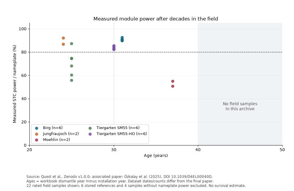
Display every rated field sample in the archived workbook, including the weaker modules. Exposure is the workbook’s dismantle minus installation year, not the paper’s broad age description. Missing ratings and stored references remain in the exported audit table but are excluded from this power plot.
plot_measurements()
plt.show()
System performance loss is a separate quantity#
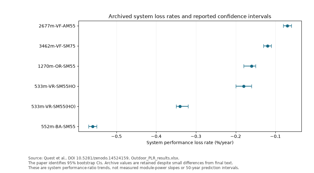
These are archived system performance-ratio loss estimates and their reported confidence intervals. They are not substituted for module-power coefficients.
plot_system_rates()
plt.show()
Project from long-exposed module groups to year 50#
Dots are measured group medians. All lines start at those ages and extrapolate a constant average loss inferred from the nameplate. They are not measured historical trajectories or longitudinal fits. Age-30 values are not fabricated for groups whose only measurement occurs later.
print(field_anchors().to_string(index=False))
plot_field_projections()
plt.show()
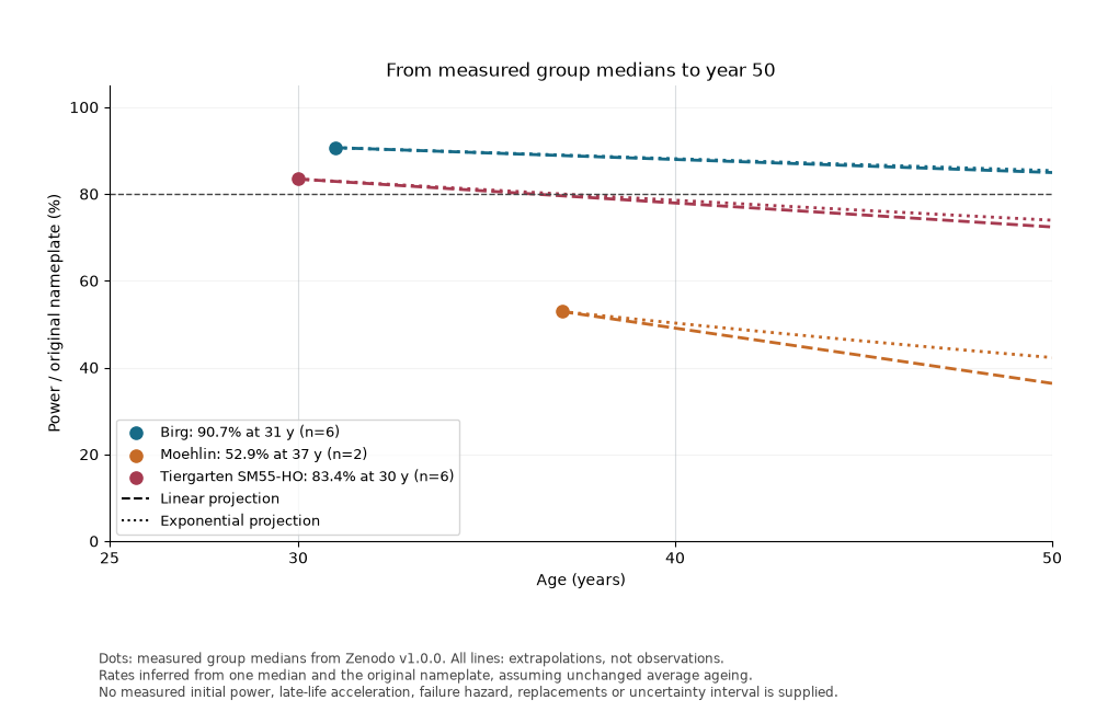
             group  age_years  retained_power  sample_count
              Birg       31.0        0.906574             6
           Moehlin       37.0        0.528977             2
Tiergarten SM55-HO       30.0        0.834324             6
A 30-year point does not fix the late-life shape#
Every curve here is hypothetical, with 90% power at year 30. Sigmoid shape B changes late-life acceleration. An unreached 80% threshold is censored at 50 years, not recorded as an infinite or exactly 50-year lifetime.
plot_shape_scenarios()
plt.show()
print(horizon_summary(shape_scenarios()).to_string(index=False))
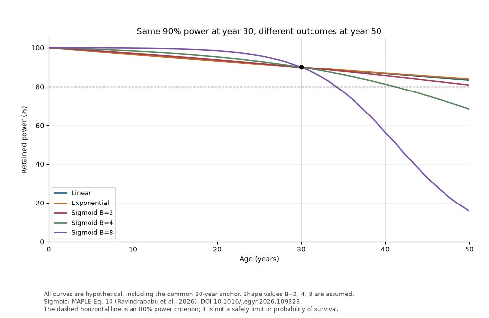
   scenario  power_at_30_percent  power_at_40_percent  power_at_50_percent  threshold_crossing_year        threshold_status                                      evidence
     Linear                 90.0            86.666667            83.333333                      NaN  not reached by year 50 hypothetical scenario, not a field prediction
Exponential                 90.0            86.894045            83.895278                      NaN  not reached by year 50 hypothetical scenario, not a field prediction
Sigmoid B=2                 90.0            85.641829            80.770378                      NaN  not reached by year 50 hypothetical scenario, not a field prediction
Sigmoid B=4                 90.0            81.232204            68.381861                41.116915 reached within 50 years hypothetical scenario, not a field prediction
Sigmoid B=8                 90.0            56.445700            15.756268                34.181339 reached within 50 years hypothetical scenario, not a field prediction
Preserve damage when stress changes#
Selected MAPLE equations: normalized sigmoid power (Eq. 10), equivalent time (Eq. 13) and independent mode multiplication (Eq. 8). The rate multipliers and background rate are assumptions, not inferred climate projections. Previously accumulated damage remains when elevated stress ends at year 40.
plot_stress_scenarios()
plt.show()
print(horizon_summary(stress_scenarios()).to_string(index=False))
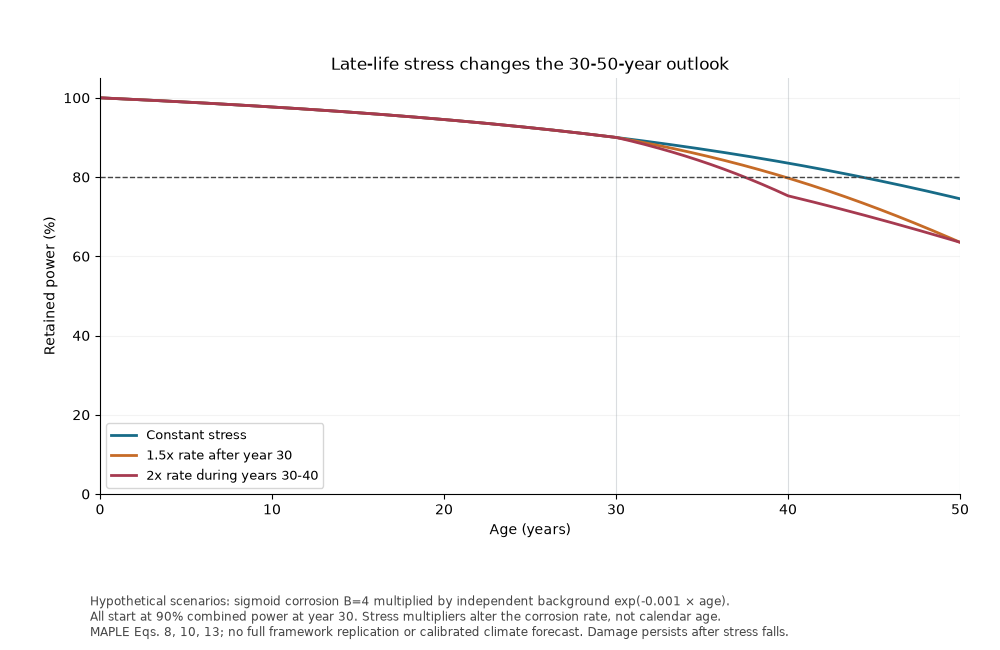
                  scenario  power_at_30_percent  power_at_40_percent  power_at_50_percent  threshold_crossing_year        threshold_status                                      evidence
           Constant stress                 90.0            83.518734            74.516804                44.275795 reached within 50 years hypothetical scenario, not a field prediction
   1.5x rate after year 30                 90.0            79.753452            63.534947                39.811807 reached within 50 years hypothetical scenario, not a field prediction
2x rate during years 30-40                 90.0            75.265711            63.534947                37.472850 reached within 50 years hypothetical scenario, not a field prediction
Inspect the complete 30-50-year design window#
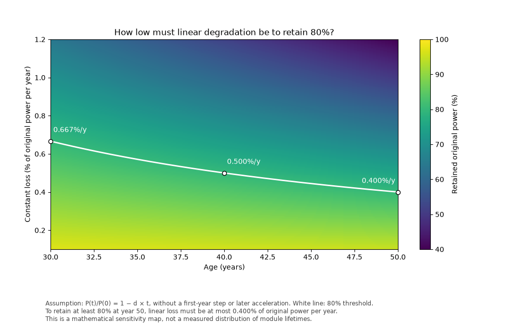
This mathematical sensitivity map answers how low a constant linear loss must be to retain 80% original power. At 50 years the maximum is 0.4%/year; an exponential model would use a different coefficient and threshold relation.
plot_rate_thresholds()
plt.show()
Total running time of the script: (0 minutes 0.569 seconds)