Note
Go to the end to download the full example code.
HVAC: shifted starts and counterfactual response#
Reproduce Foobot’s T2 comparison for starts shifted by -60, -30, +30 and +60 minutes. Each intervention is paired with the same morning’s T2 zero-offset forecast, never with T1, which has a different issue time. Setpoints stay fixed.
Data are imported publisher EnergyPlus/Timestral outputs. The original EnergyPlus model and inference are not rerun. See the Foobot article.
Shift error = (predicted candidate - predicted baseline comfort time) minus (simulated candidate - simulated baseline comfort time). Negative error means underestimated delay. Missing comfort events remain censored and counts are reported. Sensitivity slopes use only complete five-schedule mornings.
from pathlib import Path

import matplotlib.pyplot as plt
import numpy as np
import pandas as pd

root = (
    Path(globals().get("__file__", "plot_thermal_counterfactual.py")).resolve().parent
    / "data"
    / "thermal"
)
scores = pd.read_csv(root / "thermal_scores.csv")
sensitivity = pd.read_csv(root / "thermal_sensitivity.csv")
t2 = scores[(scores.test == "T2") & (scores.offset_min != 0)]
summary = t2.groupby("offset_min").shift_error_min.agg(
    valid="count", signed_mean="mean", mae=lambda x: x.abs().mean()
)
print(summary.to_string())
print(f"Valid pairs: {t2.shift_error_min.notna().sum()} / {len(t2)}")
print(f"Mean absolute shift error: {t2.shift_error_min.abs().mean():.1f} min")
print(f"Complete sensitivity days: {sensitivity.valid.sum()} / {len(sensitivity)}")
print(f"Median slope ratio: {sensitivity.sensitivity_ratio.median():.2f}")
fig, axes = plt.subplots(1, 2, figsize=(11, 4), layout="constrained")
axes[0].bar(summary.index.astype(str), summary.mae, color="#d77739")
axes[0].set(xlabel="HVAC start offset (min)", ylabel="Mean absolute shift error (min)")
valid = sensitivity[sensitivity.valid]
axes[1].scatter(valid.truth_slope, valid.prediction_slope, color="#167d9a")
limit = max(valid.truth_slope.max(), valid.prediction_slope.max()) * 1.1
axes[1].plot([0, limit], [0, limit], "--", color="gray", label="Equal response")
axes[1].set(xlabel="EnergyPlus slope (min/min)", ylabel="Timestral slope (min/min)")
axes[1].legend()
fig.suptitle("Published simulations: forecast response to changed heating starts")
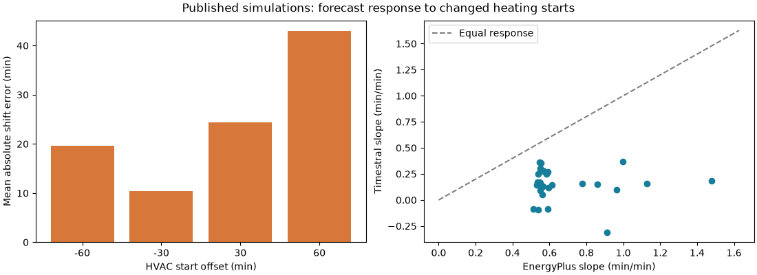
            valid  signed_mean        mae
offset_min
-60            29    17.616035  19.646647
-30            29     8.881872  10.447397
 30            30   -24.338261  24.338261
 60            29   -42.994968  42.994968
Valid pairs: 117 / 120
Mean absolute shift error: 24.4 min
Complete sensitivity days: 29 / 30
Median slope ratio: 0.23
January 12 reveals the mechanism: the delayed forecast warms before enablement. Pointwise q10-q90 temperature bands are NOT comfort-time confidence intervals.
trajectory = pd.read_csv(root / "thermal_january12.csv")
fig, axes = plt.subplots(1, 2, figsize=(11, 4), layout="constrained", sharey=True)
for ax, (offset, frame) in zip(axes, trajectory.groupby("offset_min"), strict=True):
    ax.plot(frame.minute, frame.truth_c, label="EnergyPlus (published)")
    ax.plot(frame.minute, frame.median_c, label="Timestral median (published)")
    ax.fill_between(frame.minute, frame.q10_c, frame.q90_c, alpha=0.2, label="Pointwise q10-q90")
    ax.axhline(20.75, linestyle=":", color="gray")
    ax.axvline(offset, linestyle="--", color="black", label="HVAC available")
    ax.set(
        title=f"Start offset: {offset:+d} min",
        xlim=(-60, 180),
        xlabel="Minutes relative to baseline start",
        ylabel="Temperature (°C)",
    )
axes[0].legend(fontsize=8)
fig.suptitle("January 12 — fixed setpoints, changed HVAC availability")
day = scores[(scores.date == "2024-01-12") & (scores.test == "T2")]
print(
    day[["offset_min", "prediction_met_min", "unrestricted_prediction_met_min"]].to_string(
        index=False
    )
)
assert np.isfinite(trajectory.truth_c).all()
plt.show()
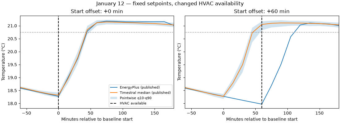
offset_min  prediction_met_min  unrestricted_prediction_met_min
       -60           41.770939                        41.770939
       -30           42.622289                        42.622289
         0           43.585766                        43.585766
        30           44.652169                        44.652169
        60           60.000000                        46.079549
Total running time of the script: (0 minutes 0.263 seconds)