Note
Go to the end to download the full example code.
Contiguous Chile KGPV: 250 m solar grid and 1 km climate#
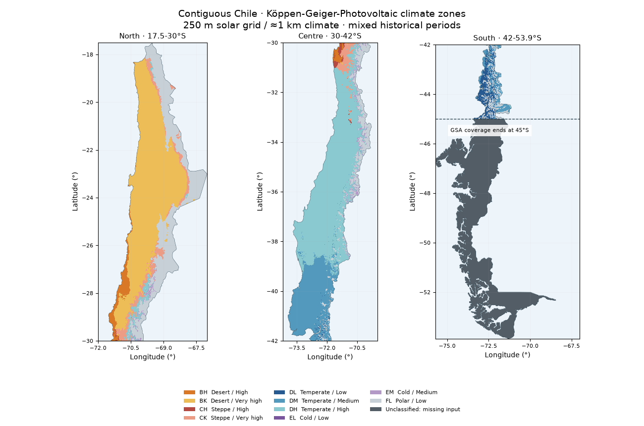
Map Chile’s connected mainland, from Arica to the Brunswick Peninsula, and zoom into the Atacama and central valleys. The GeoTIFF retains the 9-arcsecond solar grid (nominal 250 m). Temperature and rainfall retain their 30-arcsecond support (about 1 km); a finer output pixel is not finer climate information.
Coverage limit: Usable Global Solar Atlas values end at 45°S (the file rectangle reaches 46°S). Southern mainland and other cells missing any input are gray, explicitly unclassified, rather than extrapolated. This example does not claim a complete high-resolution KGPV classification of Chile. It uses the finest verified, openly downloadable GHI grid adopted here, not a proven universal maximum resolution. See the data guide.
This is an exploratory mixed-period application: CHELSA v2.1 1981-2010 and Global Solar Atlas 1999-2018. The thesis and 2019 paper supply the method, not these input datasets or an independent validation of the resulting map.
import hashlib
import json
from pathlib import Path

import matplotlib.pyplot as plt
import numpy as np
import pandas as pd
from matplotlib.patches import Patch
from matplotlib.ticker import MaxNLocator

from energy_analysis.canary_kgpv.plotting import COLORS, MISSING_COLOR, plot_tile
from energy_methods.country_boundaries import load_country_boundaries, polygons
from energy_methods.kgpv import IRRADIATION_NAMES, TP_NAMES, ZONE_CODES, classify_kgpv
Download the original pixels and boundary#
KGPV GeoTIFF contains three bands:
class ID (1-12; 0 unclassified), mainland mask (0/1), and complete-input flag
(0/1). EPSG:4326 coordinates preserve the native GSA lattice. The contour is
available as GeoJSON or Shapefile
companions (keep all five together):
.shp,
.shx,
.dbf,
.prj,
.cpg.
Also download provenance and
sample inputs. This gallery runs offline.
“Contiguous” means the largest connected Chile polygon by geodesic area. Tierra del Fuego, Chiloé, offshore islands and Antarctica are excluded. Natural Earth 1:10 million boundaries preserve holes; they are not survey contours and do not have 10 m positional accuracy.
manifest = json.loads(Path("kgpv_chile_provenance.json").read_text())
record = manifest["map"]
for file_key, hash_key in [
    ("file", "sha256"),
    ("boundary_file", "boundary_sha256"),
    ("sample_file", "sample_sha256"),
]:
    if hashlib.sha256(Path(record[file_key]).read_bytes()).hexdigest() != record[hash_key]:
        raise ValueError("Chile example file differs from its reviewed provenance")
map_path = Path(record["file"])
boundary = load_country_boundaries(Path(record["boundary_file"]), "CHL")
print(f"Classified mainland pixels: {record['classified_pixels']:,}")
print(f"Mainland pixels missing complete inputs: {record['missing_mainland_pixels']:,}")
print("Climate support ≈1 km; solar/output grid nominally 250 m. No gap filling.")
Classified mainland pixels: 7,848,061
Mainland pixels missing complete inputs: 2,621,175
Climate support ≈1 km; solar/output grid nominally 250 m. No gap filling.
Mainland overview in three adjoining latitude bands#
Colors use the repository’s fixed KGPV classes and irradiation thresholds. Only display reads are reduced; the TIFF keeps all computed pixels. The thin line shows the supplied mainland contour, not the source-data coverage edge.
present = [i for i in range(1, 13) if record["class_counts"][ZONE_CODES[i]]]
handles = [
    Patch(
        facecolor=COLORS[i - 1],
        label=(
            f"{ZONE_CODES[i]}  {TP_NAMES[ZONE_CODES[i][0]]} / {IRRADIATION_NAMES[ZONE_CODES[i][1]]}"
        ),
    )
    for i in present
]
handles.append(Patch(facecolor=MISSING_COLOR, label="Unclassified: missing input"))


def draw_mainland(ax, bounds):
    plot_tile(map_path, ax, bounds=bounds, outline=False, maximum_display_pixels=1_200_000)
    for part in polygons(boundary.geometry):
        for ring in (part.exterior, *part.interiors):
            xy = np.asarray(ring.coords)
            ax.plot(xy[:, 0], xy[:, 1], color="#455d6a", linewidth=0.4)
    ax.set(xlim=(bounds[0], bounds[2]), ylim=(bounds[1], bounds[3]))
    ax.xaxis.set_major_locator(MaxNLocator(4))
    ax.tick_params(labelsize=8)


fig, axes = plt.subplots(1, 3, figsize=(13, 8.6))
for ax, (title, bounds) in zip(
    axes,
    [
        ("North · 17.5-30°S", (-72.0, -30, -67.0, -17.505)),
        ("Centre · 30-42°S", (-74.2, -42, -69.5, -30)),
        ("South · 42-53.9°S", (-75.712, -53.887, -67.01, -42)),
    ],
    strict=True,
):
    draw_mainland(ax, bounds)
    ax.set_title(title, fontsize=11)
axes[2].axhline(-45, color="#263f4a", linestyle="--", linewidth=1)
axes[2].text(
    -74.8,
    -45.35,
    "GSA coverage ends at 45°S",
    fontsize=8,
    va="top",
    bbox={"facecolor": "white", "alpha": 0.85, "edgecolor": "none"},
)
fig.suptitle(
    "Contiguous Chile · Köppen-Geiger-Photovoltaic climate zones\n"
    "250 m solar grid / ≈1 km climate · mixed historical periods",
    fontsize=14,
)
fig.legend(handles=handles, loc="lower center", ncol=3, fontsize=8, frameon=False)
fig.subplots_adjust(top=0.90, bottom=0.20, wspace=0.23)
plt.show()
Regional detail#
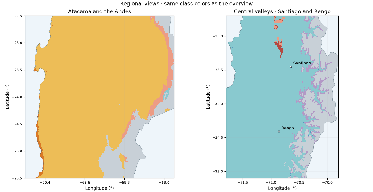
The native grid is retained without smoothing. Desert and steppe transitions depend on monthly rainfall and temperature; solar bands retain their own 250 m support. These maps are exploratory regional screening, not site-level forecasts or validated 250 m climate measurements.
fig, axes = plt.subplots(1, 2, figsize=(12, 6.2), layout="constrained")
for ax, (title, bounds) in zip(
    axes,
    [
        ("Atacama and the Andes", (-70.8, -25.5, -67.8, -22.5)),
        ("Central valleys · Santiago and Rengo", (-71.8, -35.1, -69.8, -32.7)),
    ],
    strict=True,
):
    draw_mainland(ax, bounds)
    ax.set_title(title)
for lon, lat, label in [(-70.65, -33.45, "Santiago"), (-70.86, -34.41, "Rengo")]:
    axes[1].plot(lon, lat, "o", color="white", markeredgecolor="#213a49", markersize=4)
    axes[1].annotate(label, (lon, lat), xytext=(6, 5), textcoords="offset points", fontsize=9)
fig.suptitle("Regional views · same class colors as the overview")
plt.show()
Verify sample classifications and retain the unknown area#
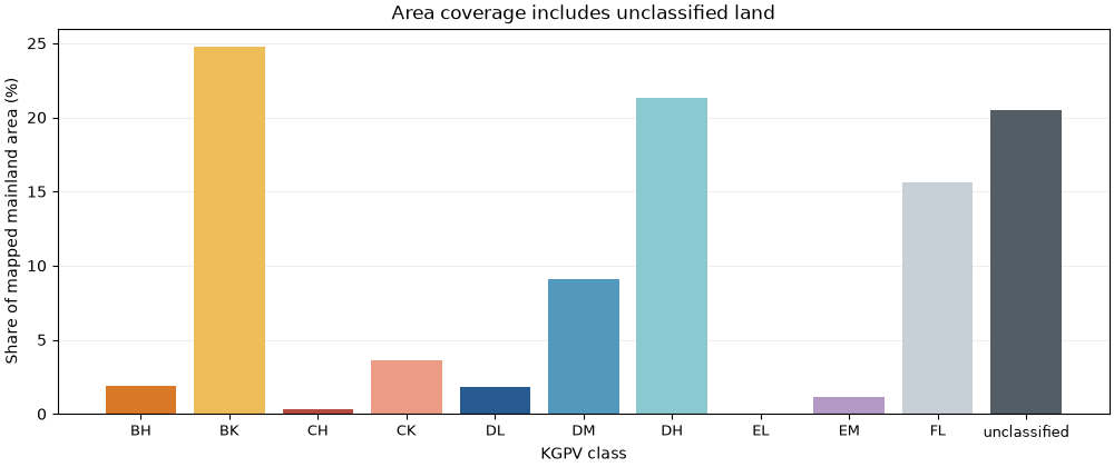
The CSV records the centre of each selected output pixel, twelve monthly temperatures (°C), twelve monthly precipitation totals (mm), annual GHI (kWh/m²) and the resulting class. GHI is already annual: multiplying it by 365 again would give incorrect results. The classifier applies Southern Hemisphere seasons and fixed global thresholds; no Chile-specific percentile thresholds are fitted. Missing GHI at Cochrane and Punta Arenas stays missing.
samples = pd.read_csv(record["sample_file"])
recomputed = classify_kgpv(
    samples[[f"tas_{m:02d}" for m in range(1, 13)]].to_numpy(),
    samples[[f"pr_{m:02d}" for m in range(1, 13)]].to_numpy(),
    samples.annual_ghi_kwh_m2.to_numpy(),
    samples.latitude.to_numpy(),
)
np.testing.assert_array_equal(recomputed.class_id, samples.class_id)
print(samples[["site", "annual_ghi_kwh_m2", "zone"]].fillna("unclassified").to_string(index=False))

areas = record["area_km2"]
keys = [ZONE_CODES[i] for i in present] + ["unclassified"]
percent = 100 * np.asarray([areas[k] for k in keys]) / sum(areas.values())
fig, ax = plt.subplots(figsize=(10, 4.2), layout="constrained")
ax.bar(keys, percent, color=[COLORS[i - 1] for i in present] + [MISSING_COLOR])
ax.set(
    ylabel="Share of mapped mainland area (%)",
    xlabel="KGPV class",
    title="Area coverage includes unclassified land",
)
ax.tick_params(axis="x", labelsize=9)
ax.grid(axis="y", alpha=0.2)
ax.set_axisbelow(True)
plt.show()
               site annual_ghi_kwh_m2         zone
              Arica       2134.885986           BK
          Altiplano       2486.987061           FL
            Atacama       2639.662109           BK
            Copiapo       2276.238037           BK
          La Serena       1730.188965           BH
           Santiago       2029.328979           DH
              Rengo       1916.467041           DH
             Temuco       1558.156006           DM
       Puerto Montt       1315.265015           DM
          Coyhaique      unclassified unclassified
           Cochrane      unclassified unclassified
Punta Arenas inland      unclassified unclassified
Attribution#
CHELSA v2.1 climatologies: Karger and colleagues, CC0; data DOI https://doi.org/10.16904/envidat.228. Solar: Global Solar Atlas 2.0, World Bank / ESMAP / Solargis, CC BY 4.0 with the provider’s additional terms retained in the provenance. Contours: Natural Earth, public domain. Cropping, nearest climate sampling and KGPV classification are modifications. The literature, unit checks, data gaps and exact reproduction command are in the mainland Chile guide.
Total running time of the script: (0 minutes 0.738 seconds)