Note
Go to the end to download the full example code.
Worldwide coverage of the repository’s connectors#
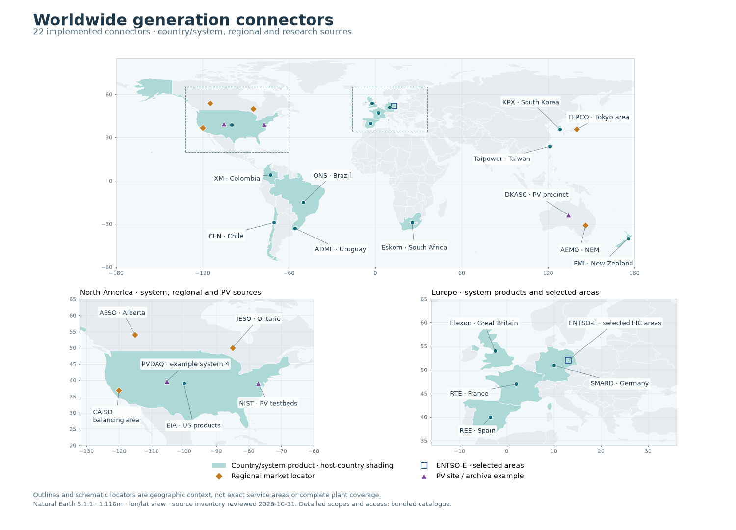
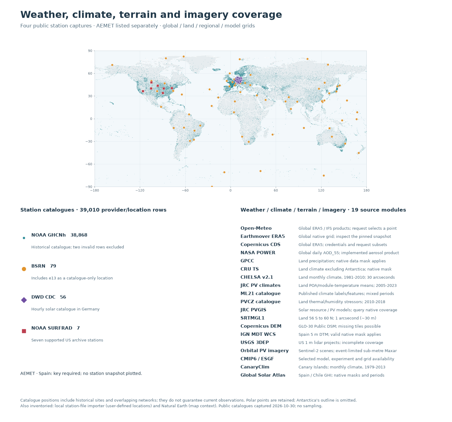
Locate all 48 source modules: 22 generation connectors, 19 gridded weather/climate/terrain/imagery sources, five station networks, a local station importer and the Natural Earth basemap. The first figure shows generation products; the second plots 39,010 provider/station catalogue rows and explains the grid products. Both figures run offline, without credentials or new downloads.
This is a map of the implemented source inventory, not a measurement of available data or exact electricity-service territories. Shaded countries are host-country context for country/system products. Diamonds locate regional markets, an open square represents selected ENTSO-E areas, and triangles mark PV research sites or one archive example. Schematic markers are not plants.
Download the connector catalogue,
world outlines,
boundary provenance,
station locations and
station provenance.
The complete examples bundle preserves
the required data/ directory alongside the Python files.
The boundaries are the public-domain Natural Earth 1:110 million countries (version 5.1.1, de facto boundaries). Every retained polygon part and vertex is unchanged. Antarctica’s unsplit ring is explicitly omitted from the basemap; Antarctic station points are retained in the second figure. These longitude / latitude views are not equal-area maps and cannot support area comparisons.
import hashlib
import json
from pathlib import Path

import matplotlib.pyplot as plt
import pandas as pd
from matplotlib.lines import Line2D
from matplotlib.patches import Patch, Rectangle

from energy_methods.country_boundaries import load_country_boundaries
from energy_methods.country_mapping import plot_country_boundaries
from energy_methods.references import get_references
1. Read the attributed offline inventory#
The catalogue records each module’s scope, access method, source references and the meaning of its locator. Its identifiers match the repository’s source directories. SHA-256 checks bind both geographic fixtures to their manifests. Country labels and regional markers are deliberately schematic; the NIST, DKASC and PVDAQ entries carry separate locator-source URLs.
directory = (
    Path(globals().get("__file__", Path.cwd() / "plot_generation_coverage.py")).resolve().parent
)
data = directory / "data"
catalogue = json.loads((data / "generation_coverage_catalogue.json").read_text(encoding="utf-8"))
boundary_manifest = json.loads(
    (data / "generation_coverage_provenance.json").read_text(encoding="utf-8")
)
station_manifest = json.loads(
    (data / "generation_coverage_stations_provenance.json").read_text(encoding="utf-8")
)
for manifest in (boundary_manifest, station_manifest):
    content = (data / manifest["fixture"]).read_bytes()
    if hashlib.sha256(content).hexdigest() != manifest["fixture_sha256"]:
        raise ValueError(f"Coverage fixture differs from its provenance: {manifest['fixture']}")

world_path = data / boundary_manifest["fixture"]
world_codes = [
    feature["properties"]["ADM0_A3"]
    for feature in json.loads(world_path.read_text(encoding="utf-8"))["features"]
]
world = load_country_boundaries(world_path, world_codes)
connectors = {item["id"]: item for item in catalogue["connectors"]}
generation = [item for item in connectors.values() if item["category"] == "generation"]
generation_country_codes = {
    code
    for item in generation
    if item["coverage_kind"] == "country_system"
    for code in item["country_codes"]
}
stations = pd.read_csv(data / station_manifest["fixture"], dtype={"station_id": str})
station_counts = stations.groupby("provider").size().to_dict()
print(f"Inventory reviewed: {catalogue['as_of']} · {len(connectors)} source modules")
print(f"Generation: {len(generation)} connectors; {len(generation_country_codes)} host countries")
print(f"Station catalogue: {len(stations):,} provider/location rows, without sampling")
Inventory reviewed: 2026-10-31 · 48 source modules
Generation: 22 connectors; 13 host countries
Station catalogue: 39,010 provider/location rows, without sampling
2. Draw generation products at their actual level of coverage#
Country shading only answers “is a country/system product implemented here?” It does not promise full national or plant coverage: EIA hourly reporting is Lower 48, Elexon is Great Britain, and RTE’s country shading does not include an overseas-data claim. SMARD implements solar and wind, KPX regional solar, and Eskom its reported owned/contracted renewables. AEMO covers the NEM, not Western Australia or the Northern Territory. CAISO, Alberta, Ontario and Tokyo-area products retain regional markers rather than country fills.
ENTSO-E takes explicitly selected EIC areas; no pan-European polygon is inferred. NIST and DKASC are native-export importers. PVDAQ’s point is example system 4, not the extent of its contributed-system archive. North America and Europe receive larger panels so every generation connector has a readable label without implying more detailed source boundaries.
COUNTRY_FILL = "#acd8d6"
SYSTEM_COLOR = "#146b75"
REGIONAL_COLOR = "#c27b20"
SITE_COLOR = "#7d4c9b"
AREA_COLOR = "#28549a"
TEXT_COLOR = "#203849"
generation_colors = {code: COUNTRY_FILL for code in generation_country_codes}
marker_styles = {
    "country_system": ("o", SYSTEM_COLOR, 34),
    "regional": ("D", REGIONAL_COLOR, 48),
    "research_site": ("^", SITE_COLOR, 60),
    "selected_areas": ("s", AREA_COLOR, 75),
}


def map_axes(ax, bounds, colors=None):
    """Reuse the repository's boundary plotting with a lon/lat view window."""
    plot_country_boundaries(world, ax=ax, colors=colors, linewidth=0.45)
    west, east, south, north = bounds
    ax.set(xlim=(west, east), ylim=(south, north), facecolor="#f3f8fb")
    ax.set_aspect("equal", adjustable="box")
    ax.tick_params(labelsize=8, colors="#60717e", length=2)
    for spine in ax.spines.values():
        spine.set_color("#cfdae1")
    ax.grid(color="#cad7df", linewidth=0.45, alpha=0.55, zorder=0)


def generation_markers(ax):
    """Each marker is a locator whose meaning is stored in the catalogue."""
    for item in generation:
        marker, color, size = marker_styles[item["coverage_kind"]]
        locator = item["locator"]
        ax.scatter(
            locator["longitude"],
            locator["latitude"],
            marker=marker,
            s=size,
            facecolor="none" if item["coverage_kind"] == "selected_areas" else color,
            edgecolor=color if item["coverage_kind"] == "selected_areas" else "white",
            linewidth=1.3 if item["coverage_kind"] == "selected_areas" else 0.6,
            zorder=4,
        )


def label_generation(ax, labels):
    """Label positions are layout choices, separate from source coordinates."""
    for provider, (label, longitude, latitude, alignment) in labels.items():
        item = connectors[provider]
        point = item["locator"]
        ax.annotate(
            label,
            xy=(point["longitude"], point["latitude"]),
            xytext=(longitude, latitude),
            ha=alignment,
            va="center",
            fontsize=9,
            color=TEXT_COLOR,
            linespacing=1.3,
            bbox={"boxstyle": "round,pad=0.25", "fc": "white", "ec": "none", "alpha": 0.9},
            arrowprops={"arrowstyle": "-", "color": "#718795", "lw": 0.7},
            zorder=5,
        )


fig_generation = plt.figure(figsize=(15, 10.8), facecolor="white")
layout = fig_generation.add_gridspec(
    2,
    2,
    height_ratios=[2.0, 1.4],
    left=0.045,
    right=0.975,
    bottom=0.16,
    top=0.89,
    hspace=0.18,
    wspace=0.09,
)
ax_world = fig_generation.add_subplot(layout[0, :])
ax_america = fig_generation.add_subplot(layout[1, 0])
ax_europe = fig_generation.add_subplot(layout[1, 1])
map_axes(ax_world, (-180, 180, -60, 85), generation_colors)
map_axes(ax_america, (-132, -60, 20, 65), generation_colors)
map_axes(ax_europe, (-16, 36, 34, 65), generation_colors)
ax_world.set(xticks=range(-180, 181, 60), yticks=range(-60, 61, 30))
for ax in (ax_world, ax_america, ax_europe):
    generation_markers(ax)
for west, south, width, height in ((-132, 20, 72, 45), (-16, 34, 52, 31)):
    ax_world.add_patch(
        Rectangle(
            (west, south),
            width,
            height,
            fill=False,
            edgecolor="#708b9a",
            linewidth=0.8,
            linestyle="--",
            zorder=3,
        )
    )

label_generation(
    ax_world,
    {
        "xm": ("XM · Colombia", -112, 2, "left"),
        "cen": ("CEN · Chile", -116, -38, "left"),
        "ons": ("ONS · Brazil", -43, 4, "left"),
        "adme": ("ADME · Uruguay", -42, -48, "left"),
        "eskom": ("Eskom · South Africa", 27, -46, "center"),
        "kpx": ("KPX · South Korea", 108, 55, "center"),
        "taipower": ("Taipower · Taiwan", 88, 15, "center"),
        "tepco": ("TEPCO · Tokyo area", 155, 44, "center"),
        "dkasc": ("DKASC · PV precinct", 112, -10, "center"),
        "aemo": ("AEMO · NEM", 142, -48, "center"),
        "emi": ("EMI · New Zealand", 179, -57, "right"),
    },
)
label_generation(
    ax_america,
    {
        "eia": ("EIA · US products", -97, 26, "center"),
        "aeso": ("AESO · Alberta", -126, 61, "left"),
        "ieso": ("IESO · Ontario", -77, 59, "center"),
        "caiso": ("CAISO\nbalancing area", -128, 29, "left"),
        "pvdaq": ("PVDAQ · example system 4", -113, 45, "left"),
        "nist": ("NIST · PV testbeds", -74, 33, "center"),
    },
)
label_generation(
    ax_europe,
    {
        "ree": ("REE · Spain", -10, 37, "left"),
        "rte": ("RTE · France", -12, 45, "left"),
        "smard": ("SMARD · Germany", 24, 47, "center"),
        "elexon": ("Elexon · Great Britain", -12, 60, "left"),
        "entsoe": ("ENTSO-E · selected EIC areas", 23, 60, "center"),
    },
)
ax_america.set_title("North America · system, regional and PV sources", loc="left", fontsize=11)
ax_europe.set_title("Europe · system products and selected areas", loc="left", fontsize=11)
fig_generation.suptitle(
    "Worldwide generation connectors",
    x=0.045,
    y=0.975,
    ha="left",
    fontsize=23,
    fontweight="bold",
    color=TEXT_COLOR,
)
fig_generation.text(
    0.045,
    0.935,
    f"{len(generation)} implemented connectors · country/system, regional and research sources",
    fontsize=12,
    color="#506b7d",
)
fig_generation.legend(
    handles=[
        Patch(facecolor=COUNTRY_FILL, label="Country/system product · host-country shading"),
        Line2D(
            [],
            [],
            marker="D",
            color="none",
            markerfacecolor=REGIONAL_COLOR,
            markeredgecolor="white",
            markersize=8,
            label="Regional market locator",
        ),
        Line2D(
            [],
            [],
            marker="s",
            color="none",
            markeredgecolor=AREA_COLOR,
            markersize=8,
            label="ENTSO-E · selected areas",
        ),
        Line2D(
            [],
            [],
            marker="^",
            color="none",
            markerfacecolor=SITE_COLOR,
            markeredgecolor="white",
            markersize=9,
            label="PV site / archive example",
        ),
    ],
    loc="lower center",
    bbox_to_anchor=(0.5, 0.083),
    ncol=2,
    frameon=False,
    fontsize=10,
    columnspacing=3.5,
)
fig_generation.text(
    0.045,
    0.045,
    "Outlines and schematic locators are geographic context, not exact service areas or complete "
    "plant coverage.\nNatural Earth 5.1.1 · 1:110m · lon/lat view · source inventory reviewed "
    f"{catalogue['as_of']}. Detailed scopes and access: bundled catalogue.",
    fontsize=9,
    color="#506b7d",
    linespacing=1.5,
)
plt.show()
3. Show station locations and keep gridded products distinct#
The public metadata captures retain every valid location in the four queried
catalogues. NOAA includes historical GHCNh sites; only two malformed source
latitudes were excluded. BSRN has 79 catalogue locations, including e13
whose numeric identifier the observation connector does not currently accept.
BSRN and SURFRAD overlap, so the total counts provider rows, not unique sites.
No catalogue point guarantees a station’s current status, variables or dates.
AEMET is listed but has no point capture here because its catalogue needs a key.
Global grids are documented product domains, not generation observations or a guarantee of a value at every location. Native masks and selected dates remain authoritative. The current NASA POWER adapter retrieves daily AOD_55; CMIP6 availability depends on the selected model, experiment and grid. CanaryClim covers the Canary Islands; the Global Solar Atlas adapter imports only its pinned Spain annual-GHI archive, not the provider’s worldwide map.
network_styles = {
    "noaa": (
        "#2f8d98",
        ".",
        3,
        0.35,
        "NOAA GHCNh",
        "Historical catalogue; two invalid rows excluded",
    ),
    "bsrn": ("#e1932c", "o", 27, 0.95, "BSRN", "Includes e13 as a catalogue-only location"),
    "dwd": ("#704fa2", "D", 18, 0.95, "DWD CDC", "Hourly solar catalogue in Germany"),
    "surfrad": ("#bc4051", "s", 27, 0.95, "NOAA SURFRAD", "Seven supported US archive stations"),
}
fig_weather = plt.figure(figsize=(15, 14), facecolor="white")
weather_layout = fig_weather.add_gridspec(
    2,
    2,
    height_ratios=[2.0, 2.4],
    left=0.045,
    right=0.975,
    bottom=0.10,
    top=0.88,
    hspace=0.20,
    wspace=0.10,
)
ax_stations = fig_weather.add_subplot(weather_layout[0, :])
ax_networks = fig_weather.add_subplot(weather_layout[1, 0])
ax_grids = fig_weather.add_subplot(weather_layout[1, 1])
map_axes(ax_stations, (-180, 180, -90, 90))
ax_stations.set(xticks=range(-180, 181, 60), yticks=range(-90, 91, 30))
for provider, (color, marker, size, alpha, _label, _scope) in network_styles.items():
    points = stations.loc[stations.provider.eq(provider)]
    ax_stations.scatter(
        points.longitude,
        points.latitude,
        s=size,
        c=color,
        marker=marker,
        alpha=alpha,
        linewidths=0 if provider == "noaa" else 0.45,
        edgecolors="white",
        rasterized=True,
        zorder=3,
        label=provider,
    )
for ax in (ax_networks, ax_grids):
    ax.set(xlim=(0, 1), ylim=(0, 1))
    ax.axis("off")

ax_networks.set_title(
    f"Station catalogues · {len(stations):,} provider/location rows",
    loc="left",
    fontsize=12,
    fontweight="bold",
    color=TEXT_COLOR,
    pad=12,
)
for row, (provider, (color, marker, _size, _alpha, label, scope)) in enumerate(
    network_styles.items()
):
    y = 0.87 - row * 0.19
    ax_networks.plot(0.018, y, marker=marker, color=color, markersize=9)
    ax_networks.text(
        0.055,
        y + 0.015,
        f"{label}   {station_counts[provider]:,}",
        fontsize=11,
        weight="bold",
        color=TEXT_COLOR,
        va="center",
    )
    ax_networks.text(0.055, y - 0.065, scope, fontsize=9.5, color="#506b7d")
ax_networks.text(
    0,
    0.03,
    "AEMET · Spain: key required; no station snapshot plotted.",
    fontsize=10,
    color=TEXT_COLOR,
)
ax_grids.set_title(
    "Weather / climate / terrain / imagery · 19 source modules",
    loc="left",
    fontsize=12,
    fontweight="bold",
    color=TEXT_COLOR,
    pad=12,
)
grid_labels = [
    ("open_meteo", "Open-Meteo", "Global ERA5 / IFS products; request selects a point"),
    ("earthmover_era5", "Earthmover ERA5", "Global native grid; inspect the pinned snapshot"),
    ("cds", "Copernicus CDS", "Global ERA5; credentials and request subsets"),
    ("nasa_power", "NASA POWER", "Global daily AOD_55; implemented aerosol product"),
    ("gpcc", "GPCC", "Land precipitation; native data mask applies"),
    ("cru_ts", "CRU TS", "Land climate excluding Antarctica; native mask"),
    ("chelsa", "CHELSA v2.1", "Land monthly climate, 1981-2010; 30 arcseconds"),
    ("jrc_climate", "JRC PV climates", "Land POA/module-temperature means; 2005-2023"),
    ("ml21", "ML21 catalogue", "Published climate labels/features; mixed periods"),
    ("pvcz", "PVCZ catalogue", "Land thermal/humidity stressors; 2010-2018"),
    ("pvgis", "JRC PVGIS", "Solar resource / PV models; query native coverage"),
    ("srtm", "SRTMGL1", "Land 56 S to 60 N; 1 arcsecond (~30 m)"),
    ("copernicus_dem", "Copernicus DEM", "GLO-30 Public DSM; missing tiles possible"),
    ("ign_terrain", "IGN MDT WCS", "Spain 5 m DTM; valid native mask applies"),
    ("usgs_3dep", "USGS 3DEP", "US 1 m lidar projects; incomplete coverage"),
    ("orbitalpv_imagery", "Orbital PV imagery", "Sentinel-2 scenes; event-limited sub-metre Maxar"),
    ("cmip6", "CMIP6 / ESGF", "Selected model, experiment and grid availability"),
    ("canary_clim", "CanaryClim", "Canary Islands; monthly climate, 1979-2013"),
    ("global_solar_atlas", "Global Solar Atlas", "Spain / Chile GHI; native masks and periods"),
]
for row, (_provider, label, scope) in enumerate(grid_labels):
    y = 0.94 - row * (0.90 / (len(grid_labels) - 1))
    ax_grids.text(0, y, label, fontsize=10.5, weight="bold", color=TEXT_COLOR, va="top")
    ax_grids.text(0.29, y, scope, fontsize=9.5, color="#506b7d", va="top")
fig_weather.suptitle(
    "Weather, climate, terrain and imagery coverage",
    x=0.045,
    y=0.975,
    ha="left",
    fontsize=23,
    fontweight="bold",
    color=TEXT_COLOR,
)
fig_weather.text(
    0.045,
    0.935,
    "Four public station captures · AEMET listed separately · "
    "global / land / regional / model grids",
    fontsize=12,
    color="#506b7d",
)
fig_weather.text(
    0.045,
    0.035,
    "Catalogue positions include historical sites and overlapping networks; they do not guarantee "
    "current observations. Polar points are retained; Antarctica's outline is omitted.\n"
    "Also inventoried: local station-file importer (user-defined locations) and Natural Earth "
    "(map context). Public catalogues captured 2026-10-30; no sampling.",
    fontsize=9,
    color="#506b7d",
    linespacing=1.5,
)
plt.show()
4. Inspect access, sources and reproducibility#
Every source module appears below and in the downloadable JSON catalogue,
which includes its full scope, references and official URL. public means
a public source, not guaranteed future endpoint availability; credential
requires provider access, export imports a user-downloaded native file,
and mixed offers more than one route. Local imports have user-defined
coverage. The worldwide provider guide
explains the generation workflows and the reference catalogue gives the full bibliographic records.
Run this file from the extracted examples bundle, or from a checkout:
uv run --all-packages python examples/connectors/plot_generation_coverage.py
To refresh public metadata deliberately from a checkout, use
scripts/prepare_connector_coverage.py and
scripts/prepare_connector_station_coverage.py. Those scripts record their
source hashes, transformations and exclusions. They never run during a normal
gallery build. The country archive is pinned; an upstream change fails its
checksum instead of silently moving borders.
inventory = pd.DataFrame(
    {
        "Module": item["id"],
        "Category": item["category"],
        "Scope type": item["coverage_kind"],
        "Access": item["access"],
    }
    for item in connectors.values()
)
print(inventory.to_string(index=False))
reference_ids = {ref for item in connectors.values() for ref in item["references"]}
reference_ids.update(boundary_manifest["reference_ids"])
reference_ids.update(station_manifest["reference_ids"])
print(f"\nAttribution validated against {len(get_references(reference_ids))} catalogue references.")
print("\nInterpretation:", catalogue["interpretation"])
            Module        Category      Scope type     Access
              adme      generation  country_system     public
             aemet station_network country_network credential
              aemo      generation        regional     public
              aeso      generation        regional      mixed
              bsrn station_network  global_network     public
             caiso      generation        regional     public
       canary_clim            grid   regional_grid     public
               cds            grid     global_grid credential
               cen      generation  country_system      mixed
            chelsa            grid       land_grid     public
             cmip6            grid  catalogue_grid     public
    copernicus_dem            grid       land_grid     public
            cru_ts            grid       land_grid     public
             dkasc      generation   research_site     export
               dwd station_network country_network     public
   earthmover_era5            grid     global_grid     public
               eia      generation  country_system      mixed
            elexon      generation  country_system     public
               emi      generation  country_system     public
            entsoe      generation  selected_areas credential
             eskom      generation  country_system     public
global_solar_atlas            grid   regional_grid     public
              gpcc            grid       land_grid     public
              ieso      generation        regional     public
       ign_terrain            grid   regional_grid     public
       jrc_climate            grid       land_grid     public
               kpx      generation  country_system credential
              ml21            grid       land_grid     public
        nasa_power            grid     global_grid     public
     natural_earth         basemap  global_basemap     public
              nist      generation   research_site     export
              noaa station_network  global_network     public
               ons      generation  country_system     public
        open_meteo            grid     global_grid     public
 orbitalpv_imagery            grid  catalogue_grid     public
              pvcz            grid       land_grid     public
             pvdaq      generation   research_site     public
             pvgis            grid       land_grid     public
               ree      generation  country_system     public
               rte      generation  country_system     public
             smard      generation  country_system     public
              srtm            grid       land_grid     public
           station    local_import    user_defined      local
           surfrad station_network country_network     public
          taipower      generation  country_system     public
             tepco      generation        regional     public
         usgs_3dep            grid   regional_grid     public
                xm      generation  country_system     public

Attribution validated against 112 catalogue references.

Interpretation: Inventory of implemented source modules, not a service-territory map or a measurement-availability test. Country shading identifies 13 host countries with country/system generation products; it does not assert complete national, plant, technology or distributed-generation coverage. Country codes follow the accompanying Natural Earth ADM0_A3 units. Regional-grid country codes identify host geography only: CanaryClim covers the Canary Islands, and the Global Solar Atlas connector retrieves only its pinned Spain annual-GHI archive. All schematic_region coordinates are illustrative country or regional locators, not provider offices, power-plant locations or coverage polygons. The PVDAQ marker is one archive example, the NIST marker is a published reference testbed and the DKASC marker is a rounded precinct locator. Global and land scope describes documented product domains only; native masks, cached catalogue bounding boxes, selected CMIP6 grids, dates and access conditions remain authoritative. The station importer has no external provider citation, and Natural Earth is geographic context rather than observed energy or weather data. Terrain grids preserve distinct product domains, native masks and vertical references; USGS 1 m is project coverage, not complete US coverage. IGN WCS is the 5 m product.
Export the figures#
The gallery provides PNG previews. Uncomment either call to export the same figures as scalable SVG for a report; dense station points are rasterized inside the vector figure to keep the file practical. No export is required to execute this example.
fig_generation.savefig(“generation_connector_coverage.svg”, bbox_inches=”tight”) fig_weather.savefig(“weather_connector_coverage.svg”, bbox_inches=”tight”, dpi=200)
Total running time of the script: (0 minutes 1.125 seconds)