Note
Go to the end to download the full example code.
California: real solar, wind and battery power#
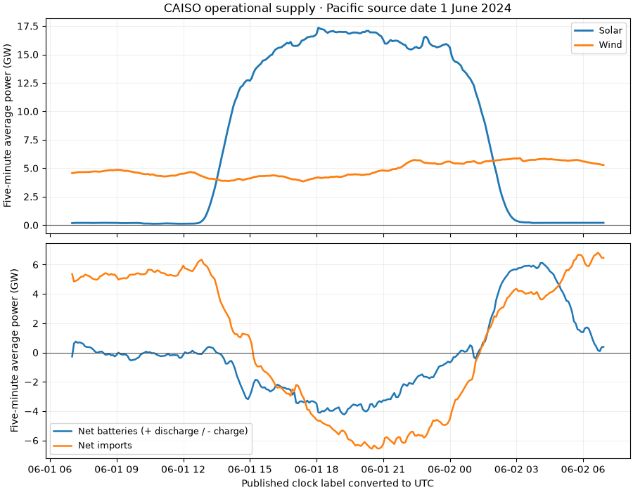
Read all 288 five-minute labels from CAISO’s native fuel-source CSV for 1 June 2024. Values are five-minute average MW. Generation, imports, net battery output and mixed Other supply remain separate. Other supply can include proxy demand response; battery charging retains its reported sign.
Source: CAISO Today’s Outlook supply. Download the
original CSV and
capture manifest.
The gallery uses this real captured file without network access or credentials.
import hashlib
import json
from datetime import date
from pathlib import Path

import matplotlib.pyplot as plt

from energy_data_retrieval.sources.caiso import parse_fuel_mix
1. Verify the native daily CSV#
For a fresh acquisition, outside the offline gallery:
from energy_data_retrieval.sources.caiso import CAISO_HOSTS, CAISOClient
from energy_data_retrieval.transport import HTTPClient
with HTTPClient(CAISO_HOSTS) as http:
    result = CAISOClient(http).generation(date(2024, 6, 1), date(2024, 6, 1))
directory = (
    Path(globals().get("__file__", Path.cwd() / "plot_generation_caiso.py")).resolve().parent
)
data = directory / "data"
manifest = json.loads((data / "generation_caiso_provenance.json").read_text())
capture = manifest["files"][0]
raw = (data / capture["file"]).read_bytes()
if hashlib.sha256(raw).hexdigest() != capture["sha256"]:
    raise ValueError("CAISO capture differs from its provenance")
print("Source:", capture["source_url"])
print("Retrieved:", capture["retrieved_at_utc"])
Source: https://www.caiso.com/outlook/history/20240601/fuelsource.csv
Retrieved: 2026-10-30T08:14:32.537560+00:00
2. Normalize source clock labels and preserve physical flows#
This ordinary June day has unambiguous Pacific clock labels. The parser rejects ambiguous/nonexistent labels on DST transition days because the native CSV does not include an offset; it never guesses a missing or repeated hour. Blank values and reported negative generation remain unchanged.
frame = parse_fuel_mix(raw.decode("utf-8"), day=date(2024, 6, 1))
print(frame.groupby("flow").agg(rows=("value", "size"), reported=("value", "count")))
profiles = frame.pivot(index="timestamp", columns="technology", values="value")
              rows  reported
flow
generation    2880      2880
net_import     288       288
net_storage    288       288
other_supply   288       288
3. Plot generation and balancing flows separately#
Batteries and imports help explain the system profile but are not additional
generating technologies. Hybrid solar/wind/battery components are already
included in their corresponding CAISO fuel categories and must not be added
again from a separate hybrid chart. Only the display unit changes to GW.
The source’s mixed Other supply is retained as flow=other_supply in the
frame, separately from generation; the charts select the four named profiles.
fig, axes = plt.subplots(2, 1, figsize=(9, 7), sharex=True, layout="constrained")
for technology, name in [("solar", "Solar"), ("wind", "Wind")]:
    axes[0].plot(profiles.index, profiles[technology] / 1000, label=name, linewidth=2)
for technology, name in [
    ("batteries", "Net batteries (+ discharge / - charge)"),
    ("imports", "Net imports"),
]:
    axes[1].plot(profiles.index, profiles[technology] / 1000, label=name, linewidth=1.8)
for ax in axes:
    ax.axhline(0, color="#555555", linewidth=0.8)
    ax.set(ylabel="Five-minute average power (GW)")
    ax.grid(alpha=0.2)
    ax.legend(fontsize=9)
axes[0].set_title("CAISO operational supply · Pacific source date 1 June 2024")
axes[1].set_xlabel("Published clock label converted to UTC")
plt.show()
Interpretation#
CAISO labels this an informational operational display, subject to change, rather than billing or settlement data. The series does not include every distributed generator and cannot establish plant-level performance losses.
Total running time of the script: (0 minutes 0.192 seconds)