Note
Go to the end to download the full example code.
Keep, repair or repower PV at year 30#
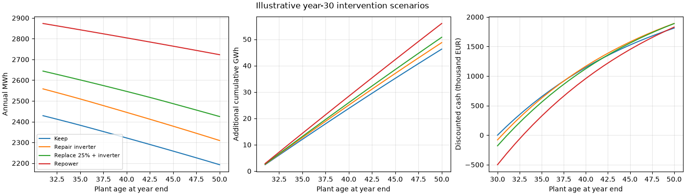
Twenty further operating years under a fixed 1 MW AC export limit. Intervention choices follow the DOE end-of-performance-period guide: https://www.energy.gov/cmei/femp/life-cycle-photovoltaic-systems-prepare-end-performance-period
Every numerical input is an illustrative assumption. The repeated hourly resource is synthetic. Module replacement resets module age at unchanged DC nameplate. Inverter repair changes assumed availability. Availability includes downtime through a uniform energy derate. Cash flows use constant real euros and a 5% real discount rate at year 30. Taxes, financing, terminal value and future resource changes are excluded.
import matplotlib.pyplot as plt
import numpy as np

from energy_methods.pv_repowering import lifetime_intervention

hour = np.arange(8760)
profile = 1.4 * np.maximum(0, np.sin(np.pi * (hour % 24 - 6) / 12))
profile *= 0.8 + 0.2 * np.cos(2 * np.pi * (hour / 24 - 172) / 365)
age = np.arange(30.5, 50)
old = 1 - 0.005 * age
new = 1 - 0.004 * (age - 30)
options = {
    "Keep": (old, 0.94, 0, 18000),
    "Repair inverter": (old, 0.99, 80000, 14000),
    "Replace 25% + inverter": (0.75 * old + 0.25 * new, 0.99, 180000, 13000),
    "Repower": (new, 0.99, 500000, 10000),
}
results = {}
fig, axes = plt.subplots(1, 3, figsize=(14, 4), layout="constrained")
for name, (retention, uptime, cost, opex) in options.items():
    frame = lifetime_intervention(
        profile,
        retention,
        ac_limit_mw=1,
        availability=np.full(20, uptime),
        price_per_mwh=70,
        annual_opex=opex,
        upfront_cost=cost,
        discount_rate=0.05,
    )
    results[name] = frame
    axes[0].plot(age + 0.5, frame.energy_mwh, label=name)
    axes[1].plot(age + 0.5, frame.cumulative_energy_mwh / 1000)
    axes[2].plot(np.arange(30, 51), np.r_[-cost, frame.cumulative_discounted_cash] / 1000)
for ax, label in zip(
    axes,
    ("Annual MWh", "Additional cumulative GWh", "Discounted cash (thousand EUR)"),
    strict=True,
):
    ax.set(xlabel="Plant age at year end", ylabel=label)
    ax.grid(alpha=0.3)
axes[0].legend(fontsize=8)
fig.suptitle("Illustrative year-30 intervention scenarios")
plt.show()
Break-even upfront intervention cost#
Discounted operating gains versus Keep define the maximum initial spend. Negative gains cannot support positive upfront expenditure.
keep_value = results["Keep"].discounted_operating_cash.sum()
for name, frame in results.items():
    ceiling = frame.discounted_operating_cash.sum() - keep_value
    print(f"{name}: break-even upfront cost versus Keep = EUR {ceiling:,.0f}")
Keep: break-even upfront cost versus Keep = EUR 0
Repair inverter: break-even upfront cost versus Keep = EUR 158,131
Replace 25% + inverter: break-even upfront cost versus Keep = EUR 256,597
Repower: break-even upfront cost versus Keep = EUR 517,042
Total running time of the script: (0 minutes 0.190 seconds)