Note
Go to the end to download the full example code.
Canary Islands KGPV: native climate pixels and 250 m solar data#
Explore all eight main islands, zoom into Tenerife, and inspect the climate inputs behind the classifications. The downloadable maps retain the current CanaryClim COG grid: about 5.2 m north-south by 4.6 m east-west. That is pixel spacing, not 5 m climate accuracy. The published CanaryClim comparison used 100 m; Global Solar Atlas irradiation remains at 9 arcseconds (nominally 250 m).
This is an exploratory application of the repository’s KGPV implementation. Temperature/rainfall cover 1979-2013 and solar irradiation 1994-2018. It is not a reconstruction of the original KGPV map or a common-period update. See the data and reproduction guide.
Run offline from examples/analysis with the accompanying files. Downloads:
provenance and
sample monthly inputs.
The full native maps contain more than 300 million classified pixels in seven
small GeoTIFFs, including La Graciosa and the other Chinijo islets:
El Hierro,
La Palma,
La Gomera,
Tenerife,
Gran Canaria,
Fuerteventura and Lobos, and
Lanzarote and Chinijo.
import hashlib
import json
from pathlib import Path

import matplotlib.pyplot as plt
import numpy as np
import pandas as pd
from matplotlib.patches import Patch
from matplotlib.ticker import MaxNLocator

from energy_analysis.canary_kgpv.plotting import COLORS, MISSING_COLOR, plot_tile
from energy_methods.kgpv import IRRADIATION_NAMES, TP_NAMES, ZONE_CODES, classify_kgpv
Verify the results and source records#
The acquisition script downloads 24 checksummed climate COGs and one solar archive, then processes native pixels in small tiles. It applies embedded scale/offset metadata and keeps source nodata. No local percentiles are fitted. Missing cells are never filled. The gallery loads the resulting rasters and recomputes eleven sample classifications below without network requests.
manifest = json.loads(Path("kgpv_canary_provenance.json").read_text(encoding="utf-8"))
for island in manifest["islands"].values():
    if hashlib.sha256(Path(island["file"]).read_bytes()).hexdigest() != island["sha256"]:
        raise ValueError("Native map checksum differs from its provenance")
samples_path = Path(manifest["sample_file"])
if hashlib.sha256(samples_path.read_bytes()).hexdigest() != manifest["sample_sha256"]:
    raise ValueError("Sample inputs differ from their provenance")
samples = pd.read_csv(samples_path)
count = sum(i["classified_pixels"] for i in manifest["islands"].values())
missing = sum(i["missing_land_pixels"] for i in manifest["islands"].values())
print(f"Native classified pixels: {count:,}; land pixels without all inputs: {missing:,}")
print("Climate: 1979-2013. Solar: 1994-2018. Mixed-period exploratory map.")
Native classified pixels: 304,733,809; land pixels without all inputs: 5,833,740
Climate: 1979-2013. Solar: 1994-2018. Mixed-period exploratory map.
The archipelago at a glance#
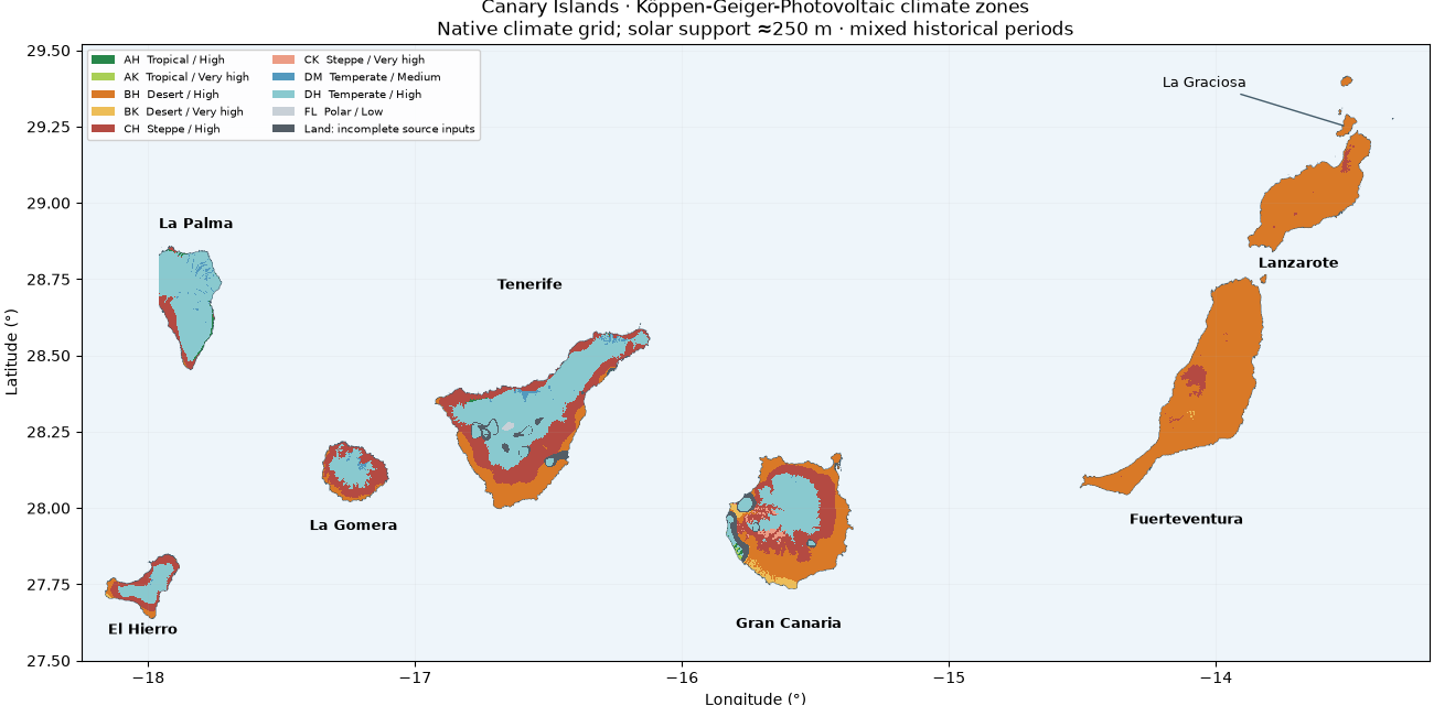
The colors and fixed thresholds are the same as the worldwide KGPV example. A bounded nearest-neighbour display read keeps this page fast; the downloadable GeoTIFFs retain every computed native pixel. Gray is missing input coverage. The outlines follow the source raster footprint, not a surveyed coastline.
present = [
    i
    for i in range(1, 13)
    if any(island["class_counts"][ZONE_CODES[i]] for island in manifest["islands"].values())
]
handles = [
    Patch(
        facecolor=COLORS[i - 1],
        label=(
            f"{ZONE_CODES[i]}  {TP_NAMES[ZONE_CODES[i][0]]} / {IRRADIATION_NAMES[ZONE_CODES[i][1]]}"
        ),
    )
    for i in present
]
handles.append(Patch(facecolor=MISSING_COLOR, label="Land: incomplete source inputs"))
labels = {
    "el_hierro": (-18.02, 27.60, "El Hierro"),
    "la_palma": (-17.82, 28.93, "La Palma"),
    "la_gomera": (-17.23, 27.94, "La Gomera"),
    "tenerife": (-16.57, 28.73, "Tenerife"),
    "gran_canaria": (-15.60, 27.62, "Gran Canaria"),
    "fuerteventura": (-14.11, 27.96, "Fuerteventura"),
    "lanzarote": (-13.69, 28.80, "Lanzarote"),
}
fig, ax = plt.subplots(figsize=(13, 6.4), layout="constrained")
for key, island in manifest["islands"].items():
    plot_tile(Path(island["file"]), ax, maximum_display_pixels=700_000)
    lon, lat, label = labels[key]
    ax.text(lon, lat, label, ha="center", va="center", fontsize=9, fontweight="bold")
ax.annotate(
    "La Graciosa",
    xy=(-13.51, 29.25),
    xytext=(-14.20, 29.38),
    fontsize=9,
    arrowprops={"arrowstyle": "-", "color": "#445c6a"},
)
ax.set(
    xlim=(-18.25, -13.20),
    ylim=(27.50, 29.52),
    title="Canary Islands · Köppen-Geiger-Photovoltaic climate zones\n"
    "Native climate grid; solar support ≈250 m · mixed historical periods",
)
ax.legend(handles=handles, loc="upper left", ncol=2, fontsize=7.5, framealpha=0.9)
plt.show()
Inspect each island#
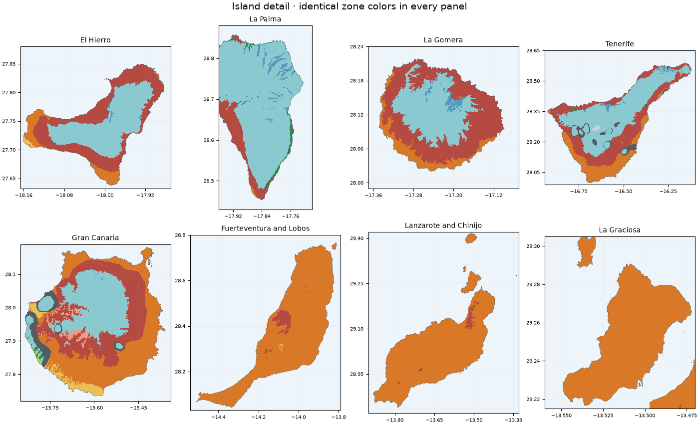
Different mountains and exposures can cross temperature/rainfall thresholds within a single solar cell. A new KGPV boundary does not imply a new solar observation. La Graciosa is shown separately from its downloadable Chinijo tile.
views = [(island["name"], Path(island["file"]), None) for island in manifest["islands"].values()]
views.append(("La Graciosa", Path("kgpv_canary_lanzarote.tif"), (-13.56, 29.215, -13.47, 29.305)))
fig, axes = plt.subplots(2, 4, figsize=(14, 8.5), layout="constrained")
for ax, (name, path, bounds) in zip(axes.flat, views, strict=True):
    plot_tile(path, ax, bounds=bounds, maximum_display_pixels=900_000)
    ax.set_title(name, fontsize=10)
    ax.tick_params(labelsize=7)
    ax.xaxis.set_major_locator(MaxNLocator(4))
    ax.yaxis.set_major_locator(MaxNLocator(5))
    ax.set_xlabel("")
    ax.set_ylabel("")
fig.suptitle("Island detail · identical zone colors in every panel", fontsize=14)
plt.show()
Zoom into native pixels on Tenerife#
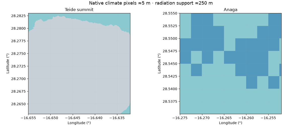
These two-kilometre-scale windows are small enough to read native pixels. The fine edges mainly reflect downscaled climate and terrain. They have not been independently validated at five metres; the GHI source stays much coarser. The square boundaries in the Anaga view expose the 250 m solar source cells.
fig, axes = plt.subplots(1, 2, figsize=(12, 5), layout="constrained")
for ax, (title, bounds) in zip(
    axes,
    [
        ("Teide summit", (-16.655, 28.263, -16.632, 28.283)),
        ("Anaga", (-16.275, 28.535, -16.252, 28.555)),
    ],
    strict=True,
):
    plot_tile(Path("kgpv_canary_tenerife.tif"), ax, bounds=bounds, maximum_display_pixels=2_000_000)
    ax.set_title(title)
fig.suptitle("Native climate pixels ≈5 m · radiation support ≈250 m", fontsize=13)
plt.show()
Recompute sample sites and explain the classification#
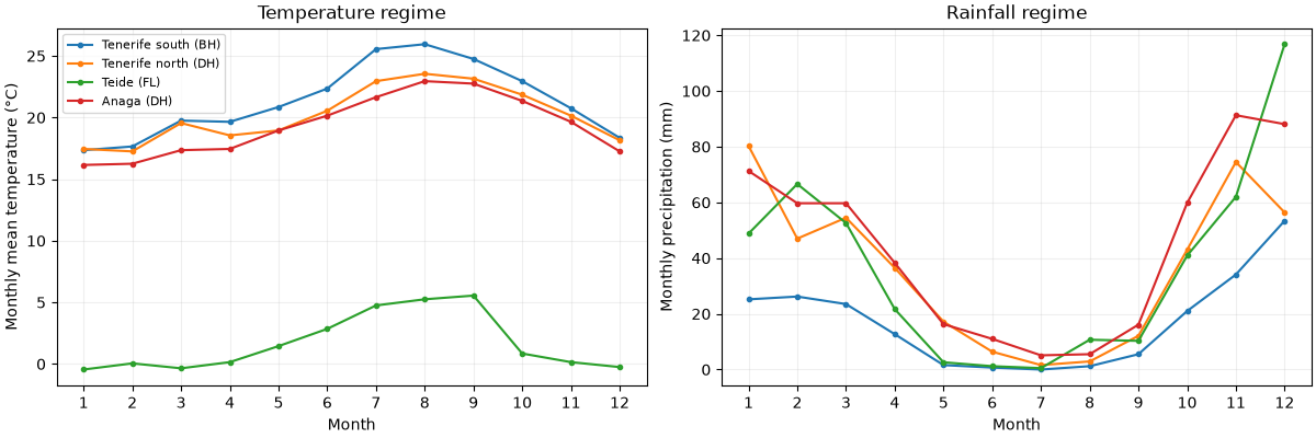
Temperature uses January-December means in °C, precipitation monthly totals
in mm, and solar annual GHI in kWh/m². The solar values are already annual
totals: multiplying them by 365 would be an error. classify_kgpv applies
the thesis/paper logic, while this application records the unequal periods.
result = classify_kgpv(
    samples[[f"t{m:02d}" for m in range(1, 13)]].to_numpy(),
    samples[[f"p{m:02d}" for m in range(1, 13)]].to_numpy(),
    samples.annual_ghi.to_numpy(),
    samples.lat.to_numpy(),
)
np.testing.assert_array_equal(result.class_id, samples.kgpv_class.to_numpy())
print(samples[["name", "annual_ghi", "kgpv_zone"]].to_string(index=False))

fig, axes = plt.subplots(1, 2, figsize=(12, 4), layout="constrained")
for name in ("Tenerife south", "Tenerife north", "Teide", "Anaga"):
    site = samples.loc[samples.name == name].iloc[0]
    axes[0].plot(
        range(1, 13),
        site[[f"t{m:02d}" for m in range(1, 13)]].astype(float),
        marker="o",
        markersize=3,
        label=f"{name} ({site.kgpv_zone})",
    )
    axes[1].plot(
        range(1, 13),
        site[[f"p{m:02d}" for m in range(1, 13)]].astype(float),
        marker="o",
        markersize=3,
        label=name,
    )
for ax in axes:
    ax.set(xlabel="Month", xticks=range(1, 13))
    ax.grid(alpha=0.2)
axes[0].set(ylabel="Monthly mean temperature (°C)", title="Temperature regime")
axes[1].set(ylabel="Monthly precipitation (mm)", title="Rainfall regime")
axes[0].legend(fontsize=8)
plt.show()
          name  annual_ghi kgpv_zone
     El Hierro 1862.775024        DH
      La Palma 1801.777954        DH
     La Gomera 1804.699951        DH
Tenerife south 1863.140015        BH
Tenerife north 1574.593018        DH
         Teide 2262.724121        FL
         Anaga 1599.430054        DH
  Gran Canaria 2000.109009        DH
 Fuerteventura 2028.598022        BH
     Lanzarote 1919.754028        BH
   La Graciosa 1845.243042        BH
Reproduce and reuse#
From the repository root, first run
uv run python scripts/prepare_kgpv_canary.py --plan-only.
Remove --plan-only to acquire approximately 1.92 GB of pinned public inputs
and recreate all native maps using bounded tile memory. Use --islands
tenerife for a single island group. Raw sources stay under artifacts/.
In each output TIFF, band 1 contains class IDs and band 2 the source footprint.
Open in QGIS or Rasterio, and retain the accompanying provenance and licenses.
The main scientific reference is Ascencio Vásquez’s doctoral thesis (2021), with the KGPV method of Ascencio-Vásquez, Brecl and Topič (2019). Climate: Karger et al. (2025), CHELSACanaryClim, CC0; Patiño et al. (2023). Solar: Global Solar Atlas 2.0, developed and operated by Solargis s.r.o. on behalf of the World Bank Group using Solargis data, funded by ESMAP. Source: https://globalsolaratlas.info, CC BY 4.0 with additional GSA terms retained in the provenance. Changes: regional extraction, sampling and KGPV derivation. No endorsement by the data providers is implied.
Total running time of the script: (0 minutes 1.944 seconds)