Note
Go to the end to download the full example code.
Map soiling and snow risk worldwide#
Apply Ascencio Vásquez (2021), equations 3.2-3.4 and Tables 6.6-6.7, to real aerosol and snow inputs. This example maps five risk levels on a coarse 15° worldwide grid for 2023, using NASA POWER AOD550 and Open-Meteo ERA5-Land physical snow depth. These are explicitly alternative sources to the thesis’s ECMWF aerosol/ERA5 inputs. One year illustrates the workflow; it is not a long-term climatology or a reproduction of the thesis’s published rasters.
Download the input CSV and
provenance JSON alongside this script.
The example runs offline, without credentials or mapping downloads:
uv sync --locked --all-packages --group docs
cd examples/analysis
uv run python plot_soiling_snow_risk.py
See the scientific guide for equations, units, boundary conventions, source preparation and interpretation.
import hashlib
import json
from pathlib import Path

import matplotlib.pyplot as plt
import numpy as np
import pandas as pd
from matplotlib.colors import BoundaryNorm, ListedColormap
from matplotlib.patches import Patch

from energy_methods.mapping import class_area_summary, write_geojson
from energy_methods.weather_risk import (
    RISK_LABELS,
    SNOW_EDGES,
    SOILING_EDGES,
    snow_loss_from_exposure,
    soiling_rate_from_aod,
)
from energy_methods.weather_risk_mapping import map_weather_risks
Load annual inputs and check their provenance#
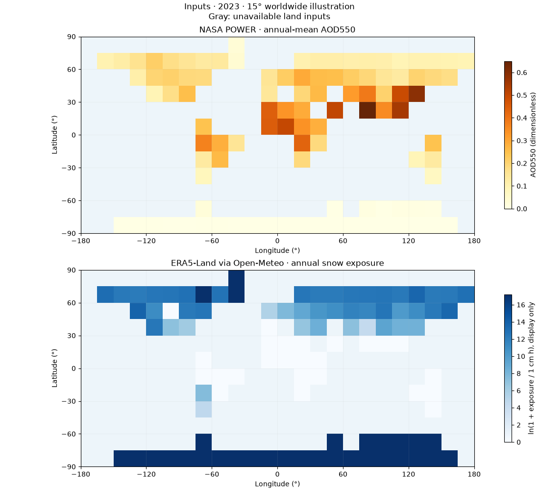
The acquisition script verifies complete UTC calendar years before reducing daily AOD to an annual mean and hourly physical snow depth to an annual sum. Blank inputs remain missing. Each indicator has its own coverage counts.
csv_path = Path("weather_risk_inputs.csv")
provenance = json.loads(Path("weather_risk_provenance.json").read_text(encoding="utf-8"))
if hashlib.sha256(csv_path.read_bytes()).hexdigest() != provenance["fixture_sha256"]:
    raise ValueError("Input fixture checksum differs from its provenance")
table = pd.read_csv(csv_path).set_index(["year", "lat", "lon"]).to_xarray()
table.aod550_mean.attrs = {"units": "1", "wavelength_nm": 550}
table.snow_depth_sum.attrs = {"units": "cm h", "snow_depth_kind": "physical_ground"}
table.attrs = {"source": provenance["description"], "fixture_sha256": provenance["fixture_sha256"]}
result = map_weather_risks(table)
land = table.is_land.isel(year=0).values == 1
spacing = provenance["grid_degrees"]
lon_edges = np.r_[table.lon.values - spacing / 2, table.lon.values[-1] + spacing / 2]
lat_edges = np.r_[table.lat.values - spacing / 2, table.lat.values[-1] + spacing / 2]
ocean_color, missing_color = "#edf5fa", "#737b83"
year = provenance["year"]


def base_map(ax):
    """Coarse centre-sampled cells; no interpolated coastlines."""
    ax.set_facecolor(ocean_color)
    ax.pcolormesh(
        lon_edges,
        lat_edges,
        np.ma.masked_where(~land, np.ones(land.shape)),
        cmap=ListedColormap([missing_color]),
        shading="flat",
    )
    ax.set(
        xlim=(lon_edges[0], lon_edges[-1]),
        ylim=(lat_edges[0], lat_edges[-1]),
        aspect="equal",
        xlabel="Longitude (°)",
        ylabel="Latitude (°)",
        xticks=np.arange(-180, 181, 60),
        yticks=np.arange(-90, 91, 30),
    )
    ax.grid(alpha=0.15, linewidth=0.6)
Inspect the two different inputs#
AOD550 is dimensionless total aerosol optical depth. Snow exposure is the sum of hourly ground snow depth in centimetres, with one-hour weights (cm h). It is neither snowfall nor snow water equivalent. A logarithmic display helps show the large snow-exposure range; zero exposure is displayed as zero.
fig, axes = plt.subplots(2, 1, figsize=(11, 10), layout="constrained")
for ax, values, title, label, cmap in (
    (
        axes[0],
        table.aod550_mean.isel(year=0).values,
        "NASA POWER · annual-mean AOD550",
        "AOD550 (dimensionless)",
        "YlOrBr",
    ),
    (
        axes[1],
        np.log1p(table.snow_depth_sum.isel(year=0).values),
        "ERA5-Land via Open-Meteo · annual snow exposure",
        "ln(1 + exposure / 1 cm h), display only",
        "Blues",
    ),
):
    base_map(ax)
    plot = ax.pcolormesh(lon_edges, lat_edges, values, cmap=cmap, vmin=0, shading="flat")
    ax.set_title(title)
    fig.colorbar(plot, ax=ax, orientation="vertical", shrink=0.75, label=label)
fig.suptitle(f"Inputs · {year} · {spacing}° worldwide illustration\nGray: unavailable land inputs")
plt.show()
Inspect the published transformations#
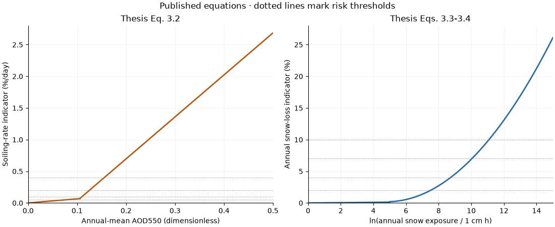
These curves illustrate equations, not observations. The soiling equation produces a daily rate in numerical %/day; multiplying it by 365 would ignore cleaning and is not an annual-loss model. The snow equation produces a numerical annual energy-loss percentage for the thesis’s fixed, latitude-tilt reference. The small discontinuities in the printed equations are retained.
fig, axes = plt.subplots(1, 2, figsize=(11, 4.5), layout="constrained")
for aod in (np.linspace(0, 0.106, 150), np.linspace(np.nextafter(0.106, 1), 0.5, 300)):
    axes[0].plot(aod, soiling_rate_from_aod(aod), color="#b25b16", linewidth=2)
for log_depth in (np.linspace(0, 5, 150), np.linspace(np.nextafter(5.0, 6), 15, 300)):
    axes[1].plot(
        log_depth, snow_loss_from_exposure(np.exp(log_depth)), color="#286b9e", linewidth=2
    )
for ax, edges in zip(axes, (SOILING_EDGES, SNOW_EDGES), strict=True):
    for edge in edges:
        ax.axhline(edge, color="#7f8b94", linestyle=":", linewidth=0.8)
    ax.grid(alpha=0.15)
    ax.spines[["top", "right"]].set_visible(False)
axes[0].set(
    xlabel="Annual-mean AOD550 (dimensionless)",
    ylabel="Soiling-rate indicator (%/day)",
    title="Thesis Eq. 3.2",
    xlim=(0, 0.5),
    ylim=(0, 2.8),
)
axes[1].set(
    xlabel="ln(annual snow exposure / 1 cm h)",
    ylabel="Annual snow-loss indicator (%)",
    title="Thesis Eqs. 3.3-3.4",
    xlim=(0, 15),
    ylim=(0, 28),
)
fig.suptitle("Published equations · dotted lines mark risk thresholds")
plt.show()
Map the five risk levels#
Apply equations to each complete year first, average annual results if there are multiple years, then classify. Exact threshold values belong to the lower class, an explicit convention where the thesis’s inequalities omit equality. Class 0 means unavailable; it is not the Very Low category. The global model products have different spatial support, so this illustration samples their nearest cells before classification rather than inventing fine-scale detail.
colors = ["#e3efb9", "#f4dc7f", "#efa950", "#d56543", "#9a3147"]
cmap = ListedColormap(colors)
norm = BoundaryNorm(np.arange(0.5, 6.5), cmap.N)
fig = plt.figure(figsize=(11, 11), layout="constrained")
grid = fig.add_gridspec(3, 1, height_ratios=[4.5, 4.5, 0.8])
for index, (name, title, units) in enumerate(
    (
        ("soiling_risk", "Soiling · thesis Table 6.7", "daily soiling-rate categories"),
        ("snow_risk", "Snow shading · thesis Table 6.6", "annual energy-loss categories"),
    )
):
    ax = fig.add_subplot(grid[index])
    base_map(ax)
    ax.pcolormesh(
        lon_edges,
        lat_edges,
        np.ma.masked_equal(result[name].values, 0),
        cmap=cmap,
        norm=norm,
        shading="flat",
    )
    ax.set_title(f"{title}\n{units}")
    print(f"{name}: {int((result[name] > 0).sum())}/{int(land.sum())} land cells classified")
legend_ax = fig.add_subplot(grid[2])
legend_ax.axis("off")
handles = [
    Patch(facecolor=color, label=label)
    for color, label in zip(colors, RISK_LABELS[1:], strict=True)
]
handles += [
    Patch(facecolor=ocean_color, edgecolor="#c3d4df", label="Ocean (masked)"),
    Patch(facecolor=missing_color, label="Unavailable land inputs"),
]
legend_ax.legend(handles=handles, loc="center", ncol=4, frameon=False, fontsize=9)
fig.suptitle(
    f"Soiling and snow risk · {year} · {spacing}° illustration\n"
    "Empirical screening, not event probabilities"
)
plt.show()
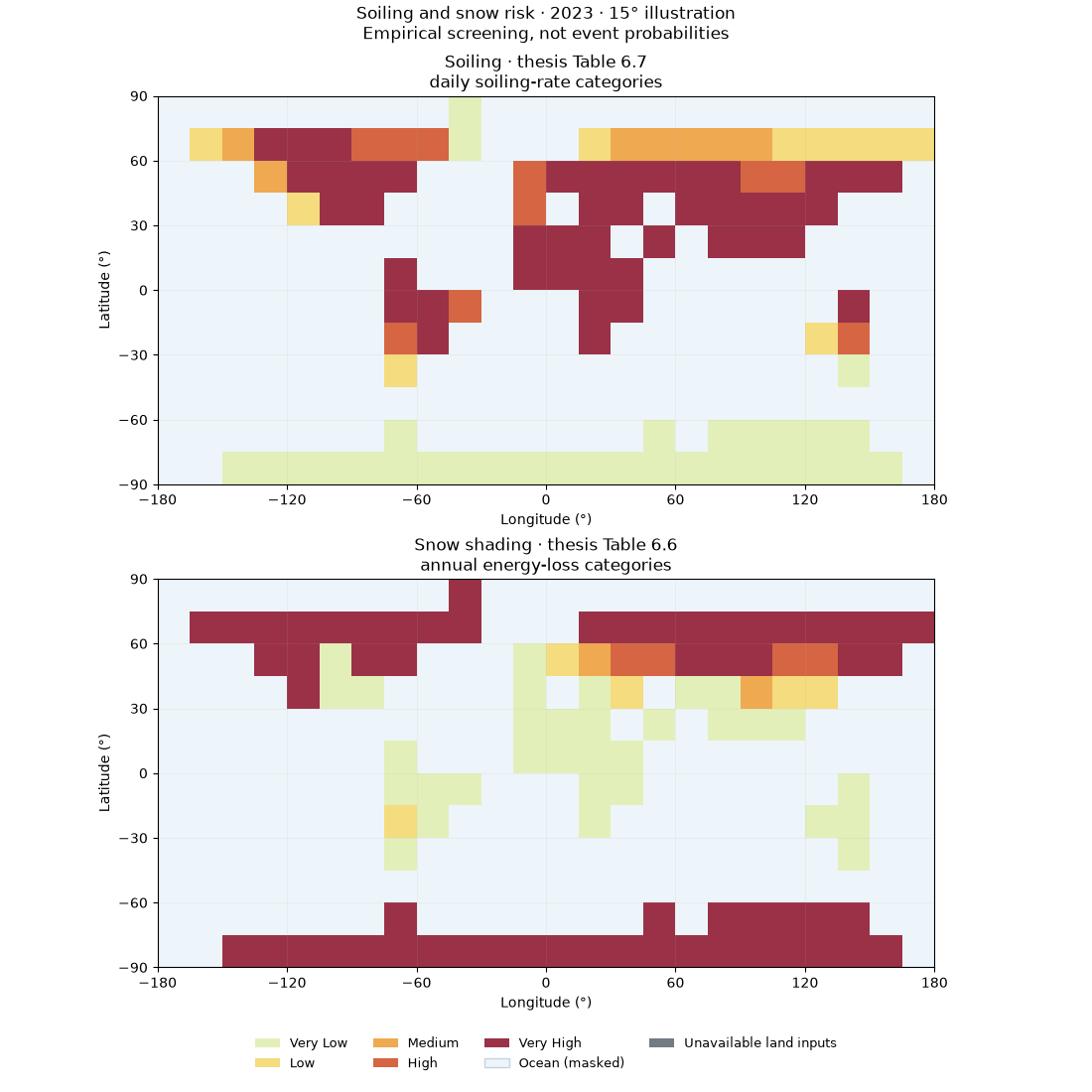
soiling_risk: 102/102 land cells classified
snow_risk: 102/102 land cells classified
Compare area shares within the classified cells#
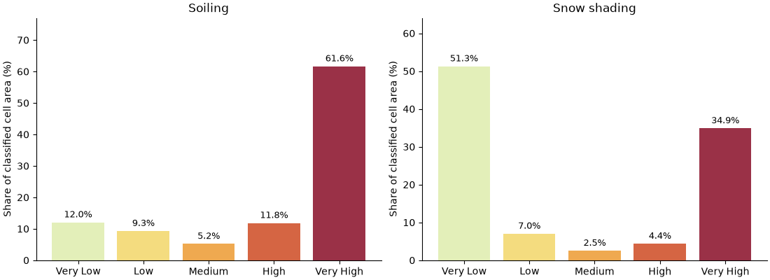
Spherical cell areas account for latitude. Each indicator uses its own available-cell denominator, excluding class 0. Coarse coastal cells count as whole cells: these are approximate cell-area shares, not land-fraction totals.
fig, axes = plt.subplots(1, 2, figsize=(11, 4), layout="constrained")
for ax, name, title in zip(
    axes, ("soiling_risk", "snow_risk"), ("Soiling", "Snow shading"), strict=True
):
    area = class_area_summary(result[name])
    total = sum(area.values())
    shares = [100 * area.get(class_id, 0) / total for class_id in range(1, 6)]
    bars = ax.bar(RISK_LABELS[1:], shares, color=colors)
    ax.bar_label(bars, fmt="%.1f%%", padding=3, fontsize=9)
    ax.set(title=title, ylabel="Share of classified cell area (%)", ylim=(0, max(shares) * 1.25))
    ax.spines[["top", "right"]].set_visible(False)
plt.show()
Export mapped indicators, classes and provenance#
Set export = True to create local files. GeoJSON polygons are grid cells,
not mapped risk contours. Annual estimates are retained in the NetCDF output.
export = False
if export:
    output = Path("soiling-snow-output")
    output.mkdir(exist_ok=True)
    result.to_netcdf(output / "soiling_snow.nc")
    for name in ("soiling_risk", "snow_risk"):
        write_geojson(
            result[name], output / f"{name}.geojson", nodata=0, labels=dict(enumerate(RISK_LABELS))
        )
    (output / "provenance.json").write_text(
        json.dumps(provenance, indent=2, ensure_ascii=False) + "\n", encoding="utf-8"
    )
Attribution and limitations#
Cite the thesis, Cordero et al. (2018) for the underlying soiling correlation, and Ryberg & Freeman (2017) for the snow modelling background. The implemented snow fit is the thesis’s adaptation, not the full SAM model. Acknowledge NASA POWER/CERES for aerosol data, Open-Meteo (CC BY 4.0), Copernicus/ERA5-Land and Muñoz-Sabater et al. (2021) for snow data, and NOAA PSL for the inherited land mask. See the bibliography.
Aerosol composition, cleaning, module geometry and local snow conditions can change actual losses. Open-Meteo warns of snow-depth overestimation. These empirical screening maps have not been independently validated against field losses and do not assess structural loading or damage.
Total running time of the script: (0 minutes 0.661 seconds)