Note
Go to the end to download the full example code.
From a reliability database to PV failure predictions#
This complete walkthrough turns a published string-inverter event rate into 30/90/365-day fleet forecasts. It shows the actual data preparation, equations, out-of-time evaluation, uncertainty and exported files. Run it offline with:
uv sync --locked --all-packages
uv run python examples/analysis/plot_pv_failure_prediction.py
The published benchmark is real. The 200-device fleet is synthetic, because the publications do not provide its underlying individual maintenance records. Results demonstrate a workflow, not validated predictions for an actual plant. The companion CLI accepts your own four CSV files; see the input guide.
1. Decide exactly what is being predicted#
We predict recurring, confirmed functional-failure events during future at-risk operating exposure. A reset alarm is not automatically a failure. A failure does not necessarily mean an inverter replacement. The model will not identify an exact failure date or rank otherwise identical devices by health. Its rate is constant within this matched cohort.
from pathlib import Path
from tempfile import TemporaryDirectory

import matplotlib.pyplot as plt
import numpy as np
import pandas as pd

from energy_analysis.pv_failure_prediction import (
    backtest,
    benchmark_prior,
    export_prediction,
    forecast_table,
    make_demo_inputs,
    plot_prediction,
    prepare_fleet,
    run_prediction,
    select_benchmark,
    split_history,
    update_from_panel,
)
from energy_data_retrieval.pv_reliability_database import load_pv_reliability_evidence
from energy_methods.failure_rates import estimate_rate
2. Inspect the source before using its number#
Filter by metric first. Availability, drift, survival and event rates have incompatible meanings. The alternative inverter rows are separate evidence, not independent observations to average. Inspect the source population, failure definition, quality flags and operating-hour convention.
rates = load_pv_reliability_evidence(metric="failure_rate")
candidate_rows = rates[rates.device == "String inverter"]
print(candidate_rows[["record_id", "value", "unit", "evidence_origin", "quality_flags"]])
benchmark = select_benchmark("baschel_2018:t1-29")
print("Selected benchmark:", benchmark)
             record_id     value  ...   evidence_origin quality_flags
26  baschel_2018:t1-27  0.000018  ...  cited_literature            []
27  baschel_2018:t1-28  0.000013  ...  cited_literature            []
28  baschel_2018:t1-29  0.000015  ...        juwi_field            []

[3 rows x 5 columns]
Selected benchmark: {'record_id': 'baschel_2018:t1-29', 'device_class': 'String inverter', 'rate_per_operating_hour': 1.51e-05, 'source_url': 'https://doi.org/10.3390/en11061579', 'source_locator': 'Table 1, PDF p. 5', 'evidence_origin': 'juwi_field', 'source_operating_hours_per_year': 4015.0, 'interpretation': 'Historical benchmark; review population and event-definition transfer.'}
3. Make the units explicit#
Baschel Table 1 supplies 15.1 events per million operating hours for the selected row. The connector stores 15.1e-6 per operating hour. Multiplying by exposure gives an expected number of events; converting to a probability requires a model. Never multiply by 8760 calendar hours when the input uses a daylight/operating clock. The paper uses 4015 operating hours/year.
source_rate = benchmark["rate_per_operating_hour"]
one_unit_hours = benchmark["source_operating_hours_per_year"]
print("Source rate per operating hour:", source_rate)
print("Expected events / source operating-year:", source_rate * one_unit_hours)
print("P(at least one event), fixed-rate Poisson:", -np.expm1(-source_rate * one_unit_hours))
Source rate per operating hour: 1.51e-05
Expected events / source operating-year: 0.0606265
P(at least one event), fixed-rate Poisson: 0.058825297112283646
4. Prepare the four tables you would obtain from SCADA and CMMS#
assets is the complete fixed-cohort asset register. exposure contains
one row for every device and observation period, including never-failed units.
events contains stable incident IDs, timestamps, event type and confirmation.
plan contains future operating hours for each device/horizon.
Here the generator creates three years of observations using a known assumed rate of 26 events/million operating hours. That hidden generating rate is NOT used by the estimator. One duplicate, one alarm, one maintenance record and one unconfirmed incident are inserted to demonstrate the audit. These are not source-paper observations.
inputs = make_demo_inputs(seed=42, devices=200)
for name, table in inputs.items():
    print(f"\n{name}: {len(table)} rows\n", table.head(3).to_string(index=False))
assets: 200 rows
 device_id    device_class
 INV-0001 String inverter
 INV-0002 String inverter
 INV-0003 String inverter

exposure: 7200 rows
 device_id              period_start                period_end  at_risk_operating_hours
 INV-0001 2023-01-01 00:00:00+00:00 2023-02-01 00:00:00+00:00                  231.862
 INV-0001 2023-02-01 00:00:00+00:00 2023-03-01 00:00:00+00:00                  241.523
 INV-0001 2023-03-01 00:00:00+00:00 2023-04-01 00:00:00+00:00                  309.150

events: 72 rows
 event_id device_id                         occurred_at         event_type  confirmed
EV-00001  INV-0006 2025-01-09 22:26:35.952775541+00:00 functional_failure          1
EV-00002  INV-0006 2025-04-20 09:55:41.559521833+00:00 functional_failure          1
EV-00003  INV-0009 2025-12-10 18:10:05.722008344+00:00 functional_failure          1

plan: 600 rows
 device_id  horizon_days  operating_hours
 INV-0001            30          231.862
 INV-0001            90          782.536
 INV-0001           365         3878.865
5. Audit the denominator and event identities#
The pipeline removes exact duplicates, rejects conflicting duplicate IDs, counts only confirmed functional failures, and retains zero-event devices. Missing exposure is rejected rather than filled with zero. Timestamps use UTC and half-open intervals [start,end), so boundary events are counted once. Operating exposure excludes down/unobservable time, with event ascertainment matched to that same scope. Software cannot verify that semantic requirement.
panel, plan, audit = prepare_fleet(inputs, device_class=benchmark["device_class"])
print("Audit:", audit)
print("Prepared panel:\n", panel.head().to_string(index=False))
print("Total at-risk device-hours:", panel.at_risk_operating_hours.sum())
Audit: {'assets': 200, 'device_periods': 7200, 'duplicate_event_rows_removed': 1, 'non_failure_or_unconfirmed_events_excluded': 3, 'confirmed_events': 68, 'never_failed_devices': 139, 'known_zero_exposure_rows': 0}
Prepared panel:
 device_id              period_start                period_end  at_risk_operating_hours  failures
 INV-0001 2023-01-01 00:00:00+00:00 2023-02-01 00:00:00+00:00                  231.862         0
 INV-0002 2023-01-01 00:00:00+00:00 2023-02-01 00:00:00+00:00                  219.800         0
 INV-0003 2023-01-01 00:00:00+00:00 2023-02-01 00:00:00+00:00                  234.910         0
 INV-0004 2023-01-01 00:00:00+00:00 2023-02-01 00:00:00+00:00                  229.105         0
 INV-0005 2023-01-01 00:00:00+00:00 2023-02-01 00:00:00+00:00                  207.390         0
Total at-risk device-hours: 2226109.755
6. Freeze a training window and hold out the future#
Fit only to 2023-2024, then evaluate on 2025. Do not randomly split rows: that would obscure whether a model would have worked at its forecast origin. The cutoff must coincide with an exposure boundary; monthly counts cannot be prorated accurately to an arbitrary date. The example uses a fixed historical as-of date, not a claim about the current state of a real fleet.
training, holdout = split_history(panel, "2025-01-01")
k_train = int(training.failures.sum())
e_train = float(training.at_risk_operating_hours.sum())
print("Training events / exposure:", k_train, e_train)
print(
    "Holdout events / exposure:", int(holdout.failures.sum()), holdout.at_risk_operating_hours.sum()
)
Training events / exposure: 42 1484073.17
Holdout events / exposure: 26 742036.585
7. Compare the raw fleet estimate with an explicit database prior#
The empirical estimate is k/E, with an exact Poisson confidence interval. The Bayesian prior is Gamma(shape=a, RATE=b), using a=2 and b=a/source_rate. Its mean equals the published rate. The strength a=2 is our assumption, not two failures or a sample size reported by the paper. Sensitivity is checked later. A source point estimate alone cannot establish prior uncertainty.
empirical = estimate_rate(k_train, e_train)
prior = benchmark_prior(benchmark, strength=2)
print("Empirical training estimate:", empirical)
print("Prior shape / rate parameter in device-hours:", prior.shape, prior.rate)
print("Prior mean and 95% rate interval:", prior.mean, prior.interval())
Empirical training estimate: RateEstimate(failures=42, exposure=1484073.17, rate=2.8300491410406674e-05, lower=2.0396504932757257e-05, upper=3.82540429448574e-05, confidence=0.95)
Prior shape / rate parameter in device-hours: 2 132450.33112582783
Prior mean and 95% rate interval: 1.51e-05 (1.8286800530069363e-06, 4.206590760158868e-05)
8. Update the rate without counting evidence twice#
Conjugate update: a_post=a+k and b_post=b+E. This combines an assumed external prior with NEW independent observations from the matched fleet. Do not also add the published table’s underlying incidents to these local observations.
fitted = update_from_panel(prior, training)
assert fitted.shape == prior.shape + k_train
assert fitted.rate == prior.rate + e_train
print("Training posterior:", fitted)
print("Updated events/million hours:", fitted.mean * 1e6)
print("Updated 95% rate interval per million hours:", np.array(fitted.interval()) * 1e6)
Training posterior: GammaRate(shape=44, rate=1616523.5011258277)
Updated events/million hours: 27.21890524285988
Updated 95% rate interval per million hours: [19.77729822 35.83042113]
9. Predict the withheld year before looking at its outcomes#
Compare the unchanged database prior against the training-updated model. Neither sees any 2025 outcomes during prediction. We report count MAE, mean negative log predictive probability (lower is better), and descriptive coverage of marginal 95% intervals. Twelve synthetic periods are not proof of field calibration. The test uses REALIZED holdout operating exposure, so it evaluates event prediction conditional on exposure, not exposure forecasting.
held_predictions, scores = backtest(prior, fitted, holdout)
print("Frozen holdout predictions:\n", held_predictions.head(6).to_string(index=False))
print("Holdout comparison:\n", scores.to_string(index=False))
Frozen holdout predictions:
              period_start          model  exposure_hours  observed_events  expected_events  count_lower  count_upper  negative_log_probability  absolute_error  interval_covers_observed
2025-01-01 00:00:00+00:00 database_prior       44355.858                1         0.669773            0            3                  1.267355        0.330227                      True
2025-02-01 00:00:00+00:00 database_prior       46204.020                0         0.697681            0            3                  0.598490        0.697681                      True
2025-03-01 00:00:00+00:00 database_prior       59141.154                2         0.893031            0            4                  1.990580        1.106969                      True
2025-04-01 00:00:00+00:00 database_prior       66533.797                4         1.004660            0            4                  3.586657        2.995340                      True
2025-05-01 00:00:00+00:00 database_prior       73926.437                3         1.116289            0            4                  2.580596        1.883711                      True
2025-06-01 00:00:00+00:00 database_prior       81319.076                6         1.227918            0            5                  4.810574        4.772082                     False
Holdout comparison:
                 model  periods  mean_absolute_error  mean_negative_log_probability  marginal_interval_coverage
       database_prior       12             1.633718                       2.122252                    0.916667
updated_from_training       12             1.404662                       1.825088                    1.000000
10. Refit as of 1 January 2026, then forecast planned exposure#
Only now do we incorporate 2025 into the posterior. Planned hours, not just a calendar horizon, drive each forecast. A shared cohort rate means device differences below come only from planned exposure, not inferred health.
current = update_from_panel(fitted, holdout)
device_forecasts = forecast_table(current, plan)
print("Per-device forecasts:\n", device_forecasts.head(6).to_string(index=False))
Per-device forecasts:
 device_id  horizon_days  operating_hours  expected_events  probability_at_least_one_event  count_lower  count_upper
 INV-0001            30          231.862         0.006881                        0.006858            0            0
 INV-0001            90          782.536         0.023225                        0.022954            0            0
 INV-0001           365         3878.865         0.115121                        0.108658            0            1
 INV-0002            30          219.800         0.006523                        0.006502            0            0
 INV-0002            90          741.824         0.022017                        0.021773            0            0
 INV-0002           365         3677.065         0.109132                        0.103312            0            1
11. Distinguish expected events, affected devices and uncertainty#
For total future exposure H, expected events are H*a/b. The chance of at least one event is 1-(b/(b+H))**a. The full predictive event-count distribution is negative-binomial: it includes BOTH uncertain rate and random future events. Multiplying rate credible limits by H does not produce a count prediction interval. For the fleet, sum H first because all devices share rate uncertainty. Do not add per-device upper bounds or assume marginal independence.
annual = device_forecasts[device_forecasts.horizon_days == 365]
future_hours = float(annual.operating_hours.sum())
print("Database-only fixed-rate expected events:", source_rate * future_hours)
print("Updated expected repeat events:", current.expected_failures(future_hours))
print("Updated 95% predictive count interval:", current.predictive_count_interval(future_hours))
print("Expected devices with >=1 event:", annual.probability_at_least_one_event.sum())
print("P(at least one event in the whole fleet):", current.probability_at_least_one(future_hours))
Database-only fixed-rate expected events: 11.204752388200003
Updated expected repeat events: 22.02299659251883
Updated 95% predictive count interval: (12, 33)
Expected devices with >=1 event: 20.835977928708672
P(at least one event in the whole fleet): 0.9999999951681126
12. Check sensitivity and turn the numbers into a bounded decision#
Re-run assumed prior strengths 0.5, 2 and 10, holding the chosen source fixed. A strong dependence on prior strength means the local evidence is still weak. Predictions can inform inspection workload or scenario budgets. They do NOT directly specify spare-inverter stock: failures may be resettable/repairable, and procurement needs repair times, lead times and replacement probabilities. If monitoring completeness, cohort homogeneity or the constant-rate assumption fails, repair the data/model before treating the forecasts as operational.
study = run_prediction(inputs, train_end="2025-01-01", input_origin="synthetic_demo")
print("Prior-strength sensitivity:\n", study["sensitivity"].to_string(index=False))
print("Fleet forecasts:\n", study["forecasts"].to_string(index=False))
figure = plot_prediction(study)
plt.show()
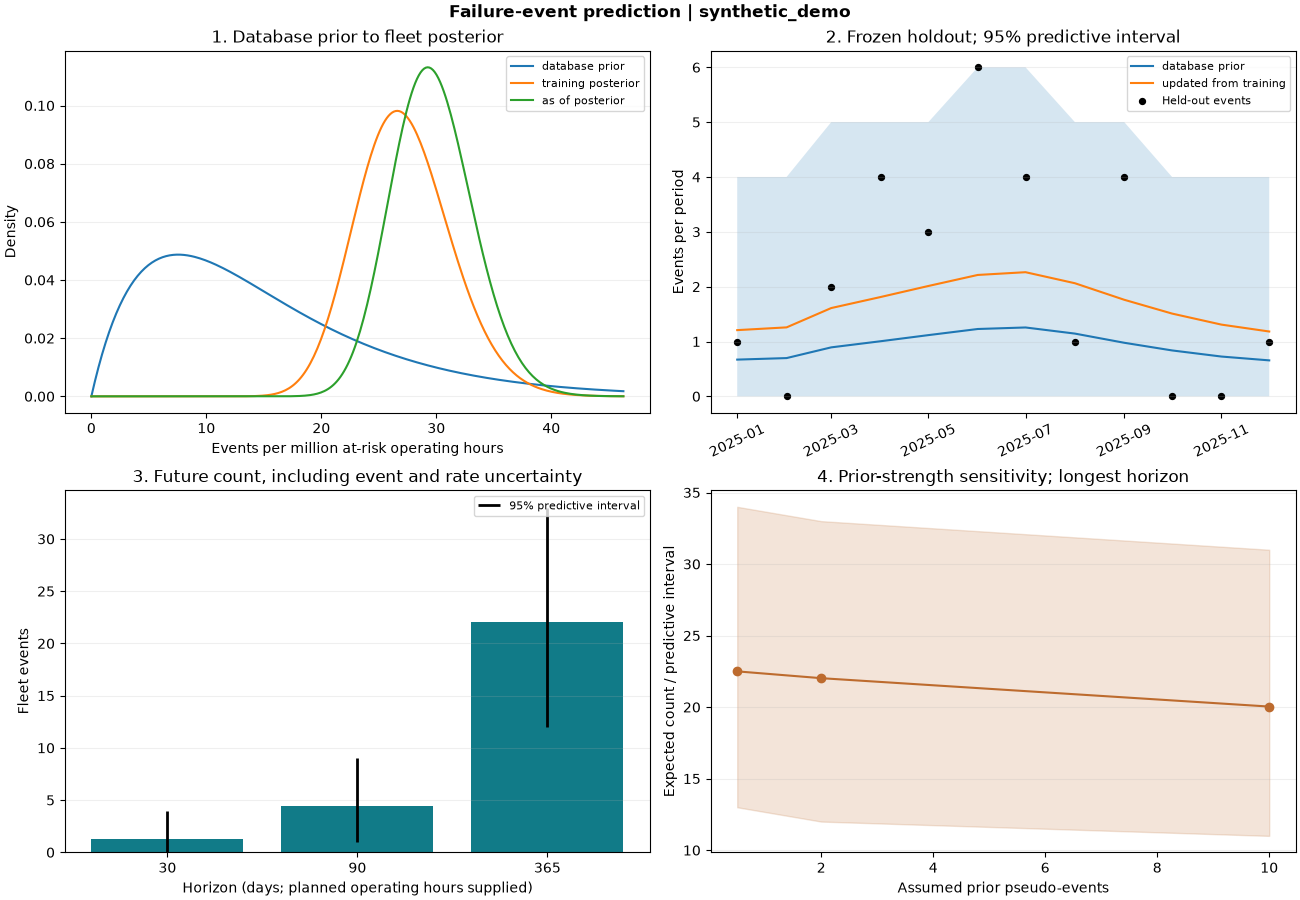
Prior-strength sensitivity:
  prior_strength  rate_per_million_hours  horizon_days  expected_events  count_lower  count_upper
            0.5               30.320168           365        22.498674           13           34
            2.0               29.679125           365        22.022997           12           33
           10.0               27.004931           365        20.038647           11           31
Fleet forecasts:
  horizon_days  devices  exposure_hours  expected_events  count_lower  count_upper  probability_any_fleet_event  expected_devices_with_event
           30      200       44355.858         1.316443            0            4                     0.728615                     1.312049
           90      200      149701.035         4.442996            1            9                     0.986535                     4.393217
          365      200      742036.582        22.022997           12           33                     1.000000                    20.835978
13. Save the inputs, audit trail and predictions#
The CLI writes persistent artifacts; this gallery uses a temporary directory to avoid changing the repository while its examples run. Four CSV inputs, seven result tables, a JSON manifest with input SHA-256 checksums, and a figure make every quantity traceable. The source record and assumed prior strength remain in the manifest. No credentials or live network calls are required.
with TemporaryDirectory() as temporary:
    output = Path(temporary)
    export_prediction(study, inputs, output)
    print(
        "Exported files:",
        sorted(str(p.relative_to(output)) for p in output.rglob("*") if p.is_file()),
    )
    reloaded = {name: pd.read_csv(output / "inputs" / f"{name}.csv") for name in inputs}
    repeated = run_prediction(reloaded, train_end="2025-01-01")
    pd.testing.assert_frame_equal(study["forecasts"], repeated["forecasts"])
    print("CSV round-trip reproduces every forecast.")
Exported files: ['devices.csv', 'failure_prediction.png', 'forecasts.csv', 'holdout.csv', 'inputs/assets.csv', 'inputs/events.csv', 'inputs/exposure.csv', 'inputs/plan.csv', 'panel.csv', 'rates.csv', 'run_manifest.json', 'scores.csv', 'sensitivity.csv']
CSV round-trip reproduces every forecast.
14. Replace the synthetic fleet with your own records#
First generate editable example input files and persistent results:
uv run python -m energy_analysis.pv_failure_prediction --output artifacts/pv-prediction
Replace all four files in a separate input directory, review the benchmark definition/population, then run with an explicit holdout boundary:
uv run python -m energy_analysis.pv_failure_prediction \
    --input-dir my_fleet --train-end 2025-01-01 \
    --benchmark-record baschel_2018:t1-29 --prior-strength 2 \
    --output artifacts/my-fleet-prediction
Run separate matched cohorts for different device classes. Do not transfer inverter rates to tracker motors or pyranometers. If individual first-failure ages are available, the repository also provides Kaplan-Meier, censored Weibull and conditional lifetime risk; a published point rate cannot identify ageing.
Total running time of the script: (0 minutes 0.968 seconds)