Note
Go to the end to download the full example code.
Perovskite-silicon tandem: what premium could extra rooftop yield justify?#
November 10, 2026 news: Heliene and Caelux announced commercial-scale production of a silicon-perovskite tandem module with efficiency up to 27%+, and a developer-claimed up to 20% energy gain versus conventional N-type silicon modules. Deliveries are planned for 2027. Those are company statements, not independently measured annual production or a bankability assessment.
Business case: how much additional upfront installed cost per occupied square metre can a higher-efficiency module justify for an area-constrained project, conditional on future degradation and the price of delivered energy?
Evidence: Heliene / Caelux release (10 November 2026): https://www.globenewswire.com/news-release/2026/11/10/3399606/0/en/heliene-and-caelux-bring-next-generation-hybrid-tandem-solar-modules-to-u-s-commercial-manufacturing.html NREL PVWatts Version 5 (Dobos, 2014, NREL/TP-6A20-62641): https://doi.org/10.2172/1158421 Jordan and Kurtz (2013), review of historical PV degradation: https://doi.org/10.1002/pip.1182
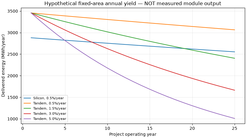
Input provenance: Only the ~27% tandem module efficiency and the up-to 20% gain announcement are sourced from the manufacturer. The conventional 22.5% module, 10,000 m² occupied module area, effective POA of 1,600 kWh/m²/year, uniform 0.80 AC delivery factor, energy price $0.08/kWh, 25-year horizon, 8% real discount and all tandem degradation values are illustrative assumptions, not Heliene field data, measured irradiance, pricing, warranties, or probabilities. The 0.5%/year silicon scenario is consistent with a historical literature median, not a tandem estimate.
This method is a simplified fixed-area energy balance, not PVWatts itself. It omits thermal/spectral response, clipping, orientation, site O&M, weather variability, warranty risk, financing, taxes, and capex other than the premium. The sensitivity curves represent scenarios, not confidence intervals.
import matplotlib.pyplot as plt

from energy_methods.tandem_pv_screen import compare_module_options, screen_fixed_area_pv

# All inputs below are explicit *SCENARIOS*, except the manufacturer-rated
# tandem 27% reference, interpreted as 0.27 for a screening calculation.
assumptions = {
    "module_area_m2": 10_000.0,
    "annual_effective_poa_kwh_per_m2": 1_600.0,
    "ac_delivery_factor": 0.80,
    "operating_years": 25,
    "real_discount_rate": 0.08,
    "annual_opex_usd_per_m2": 0.0,
}


def scenario(efficiency: float, degradation: float, tariff: float):
    """Project an illustrative module option with controlled shared assumptions."""
    return screen_fixed_area_pv(
        **assumptions,
        stc_module_efficiency=efficiency,
        annual_degradation_fraction=degradation,
        power_price_usd_per_kwh=tariff,
    )


silicon = scenario(0.225, 0.005, 0.08)
tandem_equal_aging = scenario(0.270, 0.005, 0.08)
reference = compare_module_options(
    silicon, tandem_equal_aging, module_area_m2=assumptions["module_area_m2"]
)
print(f"Synthetic same-PR, first-year gain: {reference.first_year_energy_gain_fraction:.1%}")
print(
    "Synthetic equal-aging break-even upfront tandem premium: "
    f"${reference.break_even_incremental_capex_usd_per_m2:.2f}/module-m²"
)
Synthetic same-PR, first-year gain: 20.0%
Synthetic equal-aging break-even upfront tandem premium: $47.23/module-m²
Plot 1: different annual degradation assumptions, not confidence bands.
fig, ax = plt.subplots(figsize=(8.2, 4.6), layout="constrained")
years = range(1, 26)
ax.plot(years, [energy / 1000 for energy in silicon.annual_ac_kwh], label="Silicon, 0.5%/year")
for rate in (0.005, 0.015, 0.03, 0.05):
    tandem = scenario(0.270, rate, 0.08)
    ax.plot(
        years,
        [energy / 1000 for energy in tandem.annual_ac_kwh],
        label=f"Tandem, {rate:.1%}/year",
    )
ax.set(
    title="Hypothetical fixed-area annual yield — NOT measured module output",
    xlabel="Project operating year",
    ylabel="Delivered energy (MWh/year)",
)
ax.legend(fontsize=8)
ax.grid(alpha=0.25)
plt.show()
Plot 2: merchant/PPA price and tandem-aging sensitivity of permissible premium.
fig, ax = plt.subplots(figsize=(8.2, 4.6), layout="constrained")
degradation_rates = [n / 1000 for n in range(5, 56, 5)]
for tariff in (0.04, 0.08, 0.12):
    base = scenario(0.225, 0.005, tariff)
    ceilings = [
        compare_module_options(
            base,
            scenario(0.270, rate, tariff),
            module_area_m2=assumptions["module_area_m2"],
        ).break_even_incremental_capex_usd_per_m2
        for rate in degradation_rates
    ]
    ax.plot([100 * r for r in degradation_rates], ceilings, marker="o", label=f"${tariff:.2f}/kWh")
ax.axhline(0, color="black", linewidth=1, linestyle="--")
ax.set(
    title="Allowable additional initial spend — synthetic degradation scenarios",
    xlabel="Assumed tandem annual degradation (%)",
    ylabel="Break-even incremental capex (real USD/module-m²)",
)
ax.legend(title="Real energy price")
ax.grid(alpha=0.25)
plt.show()
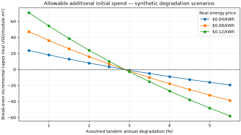
Critical caveats: reported 27%+ STC module efficiency does not imply a verified 20% annual energy uplift, even if the STC efficiency ratio of 27/22.5 happens to be exactly 1.2. No project-specific spectral, thermal, or degradation coefficients for the new product are available. Negative break-even premiums mean tandem would have LOWER discounted operating value under that illustrative aging-and-price scenario.
Reproduce (from repo root, with workspace installed): uv run –no-sync python examples/analysis/plot_heliene_caelux_tandem_2026.py
Total running time of the script: (0 minutes 0.178 seconds)